Simulate Univariate Model Responses Using Econometric Modeler App

In-sample model simulations visually demonstrate how well a model fits to a time series, particularly for stationary models, and they demonstrate the model's dynamics. This example shows how to estimate a univariate ARIMA model and simulate random paths from the model by using the Econometric Modeler app.

Although the example uses an ARIMA model, the workflow is similar for all univariate models available in Econometric Modeler, such as GARCH models.

The data set, which is stored in Data_JAustralian.mat, contains the log quarterly Australian Consumer Price Index (CPI) measured from 1972 and 1991, among other time series.

Prepare Data for Econometric Modeler

At the command line, load the Data_JAustralian.mat data set.

load Data_JAustralian

Import Data into Econometric Modeler

At the command line, open the Econometric Modeler app.

econometricModeler

Alternatively, open the app from the apps gallery (see Econometric Modeler).

Import DataTimeTable into the app:

1. On the Modeler tab, in the Import section, click the Import button .

2. In the Import Data dialog box, select the check box for the DataTimeTable variable.

3. Click Import.

The variables, including PAU, appear in the Time Series pane, and a time series plot of all the series appears in the Plot(EXCH) figure window.

Create a time series plot of PAU by double-clicking PAU in the Time Series pane.

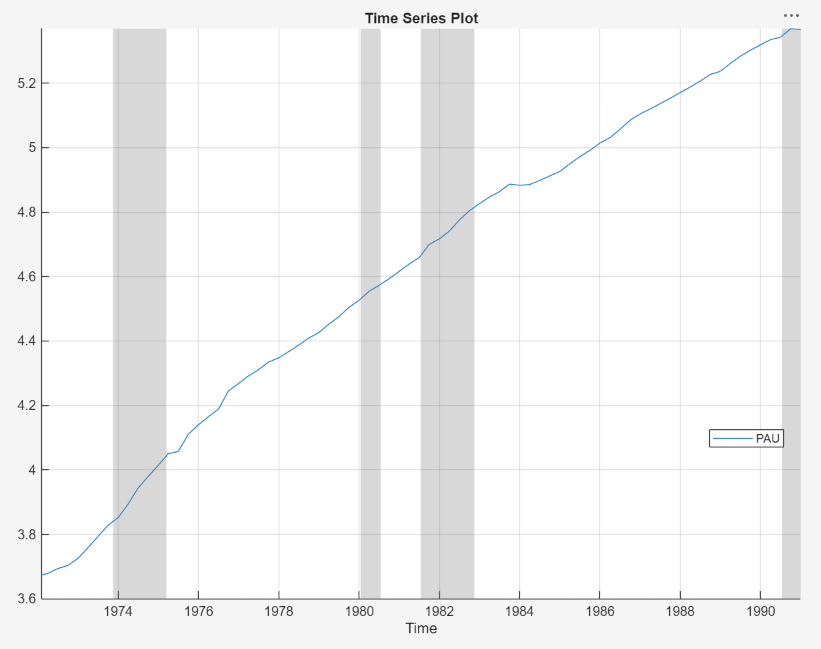
The series appears nonstationary because it has a clear upward trend.

Specify and Estimate ARIMA Model

Estimate an ARIMA(2,1,0) model containing a constant for the log quarterly Australian CPI. This model has one degree of nonseasonal differencing and two AR lags. For more details, see Implement Box-Jenkins Model Selection and Estimation Using Econometric Modeler App.

1. In the Time Series pane, select the PAU time series.

2. On the Modeler tab, in the Models section, click ARIMA.

3. In the ARIMA Model Parameters dialog box, on the Lag Order tab:

   1. Set Degree of Integration to 1.

   2. Set Autoregressive Order to 2.

   3. Set Moving Average Order to 0.

   

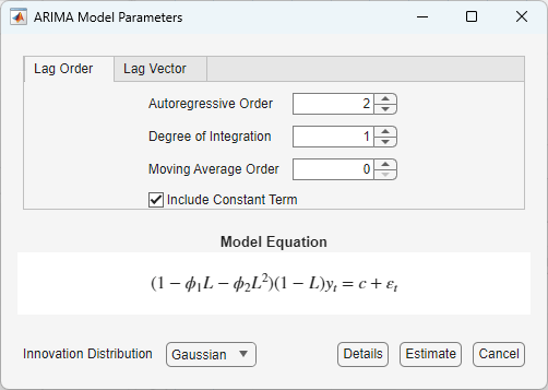
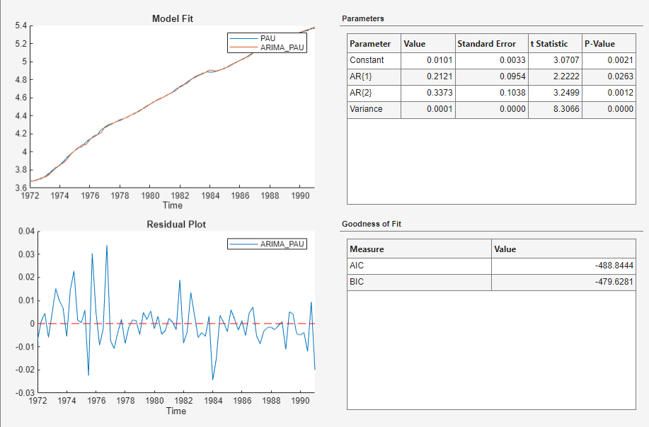
4. Click Estimate.

The model variable ARIMA_PAU appears in the Models pane, its value appears in the Preview pane, and its estimation summary appears in the Fit(ARIMA_PAU) document.

Simulate the Nonstationary Model

Determine how well a nonstationary model describes the data by simulating 100 random paths from the model.

1. In the Models pane, select the ARIMA_PAU model.

2. On the Modeler tab, in the Simulate section, click Simulate.

3. In the Simulate Model Response dialog box, set Number of simulated paths to 100. Click Simulate.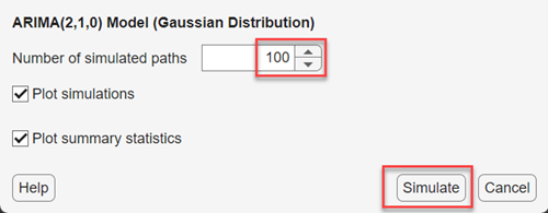

   

In the Simulations pane, a variable SIM_ARIMA_PAU appears. This variable is a structure array with the following fields:

• Simulations — T-by-k matrix of simulated paths, with rows corresponding to in-sample times and columns corresponding to the independently drawn paths

• Mean — T-by-1 vector of the pointwise average of the simulated paths

• UpperConfidenceBound — T-by-1 vector of upper confidence bounds of the pointwise 95% percentile-based confidence intervals

• LowerConfidenceBound — T-by-1 vector of lower confidence bounds of the pointwise 95% percentile-based confidence intervals

In the right pane, in the Sim(ARIMA_PAU) tab, is a plot containing the following time series:

• The time series data (thick blue line)

• Each simulated path (thin gray lines)

• The pointwise average of the simulated paths (thick orange line)

• The pointwise 95% percentile-based confidence intervals (thick orange dashed line)

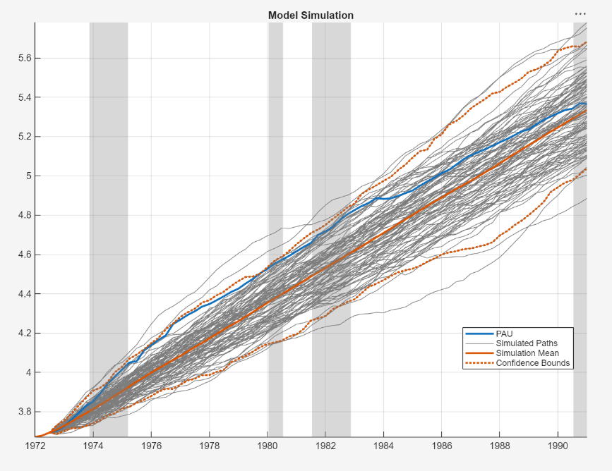
All simulated paths start at period two unless they require a longer presample to initialize the model, which is a common requirement for dynamic models. If a model requires a presample of more than 1 observation, all simulated paths begin at the time point after the end of the presample period. The length of the presample period depends on the dynamic model, see the associated reference page for details. For an AR(2) model, the presample period is two time points; therefore, all simulated paths begin at the third time point.

The time series data is always greater than the simulation mean, and mostly greater than the simulated paths. This characteristic might suggest that the model does not capture the true data-generating process well enough.

Simulate the Stationary Model

Take the first difference of the log quarterly Australian CPI time series. In the Time Series pane, select the PAU time series. Then, on the Modeler tab, in the Transforms section, click Difference.

The differenced series is PAU_Diff. A plot of the series is, on the right pane, in the Plot(PAU_Diff) tab.

Fit an AR(2) model containing a constant to the differenced series.

1. In the Time Series pane, select PAU_Diff.

2. In the Modeler tab, in the Models section, click AR.

3. In the AR Model Parameters dialog box, set Autoregressive Order (p) to 2.

4. Click Estimate.

An estimation summary appears in the Fit(AR_PAU_Diff) tab, and the estimated model AR_PAU_Diff appears in the Models pane.

Determine how well a stationary model describes the data by simulating 100 random paths from the model.

1. In the Models pane, select the AR_PAU_Diff model.

2. On the Modeler tab, in the Simulate section, click Simulate.

3. In the Simulate Model Response dialog box, set Number of simulated paths to 100.

4. Click Simulate.

In the Simulations pane, a variable SIM_AR_PAU_Diff appears. In the right pane, in the Sim(AR_PAU_Diff) tab, is a plot containing the time series data, simulated paths, and simulation statistics.

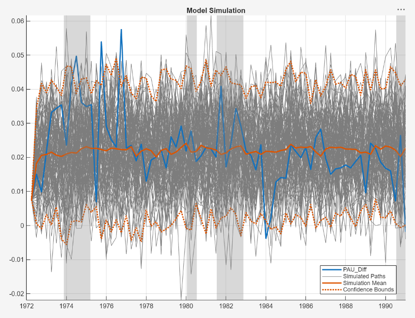
The time series data mostly stays well within the confidence intervals and oscillates around its mean, but several observations are outside the bounds.