lassoblm
Bayesian linear regression model with lasso regularization
Description
The Bayesian linear regression model object lassoblm specifies the joint prior distribution of the regression coefficients and the disturbance variance (β, σ2) for implementing Bayesian lasso regression
[1]. For j = 1,…,NumPredictors, the conditional prior distribution of βj|σ2 is the Laplace (double exponential) distribution with a mean of 0 and scale σ2/λ, where λ is the lasso regularization, or shrinkage, parameter. The prior distribution of σ2 is inverse gamma with shape A and scale B.
The data likelihood is where ϕ(yt;xtβ,σ2) is the Gaussian probability density evaluated at yt with mean xtβ and variance σ2. The resulting posterior distribution is not analytically tractable. For details on the posterior distribution, see Analytically Tractable Posteriors.
In general, when you create a Bayesian linear regression model object, it specifies the joint prior distribution and characteristics of the linear regression model only. That is, the model object is a template intended for further use. Specifically, to incorporate data into the model for posterior distribution analysis and feature selection, pass the model object and data to the appropriate object function.
Creation
Description
PriorMdl = lassoblm(NumPredictors)PriorMdl) composed of NumPredictors predictors and an intercept, and sets the NumPredictors property. The joint prior distribution of (β, σ2) is appropriate for implementing Bayesian lasso regression [1]. PriorMdl is a template that defines the prior distributions and specifies the values of the lasso regularization parameter λ and the dimensionality of β.
PriorMdl = lassoblm(NumPredictors,Name,Value)NumPredictors) using name-value pair arguments. Enclose each property name in quotes. For example, lassoblm(3,'Lambda',0.5) specifies a shrinkage of 0.5 for the three coefficients (not the intercept).
Properties
Object Functions
estimate | Perform predictor variable selection for Bayesian linear regression models |
simulate | Simulate regression coefficients and disturbance variance of Bayesian linear regression model |
forecast | Forecast responses of Bayesian linear regression model |
plot | Visualize prior and posterior densities of Bayesian linear regression model parameters |
summarize | Distribution summary statistics of Bayesian linear regression model for predictor variable selection |
Examples
Consider the multiple linear regression model that predicts the US real gross national product (GNPR) using a linear combination of industrial production index (IPI), total employment (E), and real wages (WR).
For all , is a series of independent Gaussian disturbances with a mean of 0 and variance .
Assume these prior distributions:
For j = 0,...,3, has a Laplace distribution with a mean of 0 and a scale of , where is the shrinkage parameter. The coefficients are conditionally independent.
. and are the shape and scale, respectively, of an inverse gamma distribution.
Create a prior model for Bayesian linear regression. Specify the number of predictors p.
p = 3;
Mdl = lassoblm(p);
PriorMdl is a lassoblm Bayesian linear regression model object representing the prior distribution of the regression coefficients and disturbance variance. At the command window, lassoblm displays a summary of the prior distributions.
Alternatively, you can create a prior model for Bayesian lasso regression by passing the number of predictors to bayeslm and setting the ModelType name-value pair argument to 'lasso'.
MdlBayesLM = bayeslm(p,'ModelType','lasso')
MdlBayesLM =
  lassoblm with properties:

    NumPredictors: 3
        Intercept: 1
         VarNames: {4×1 cell}
           Lambda: [4×1 double]
                A: 3
                B: 1


           |  Mean     Std           CI95         Positive   Distribution
---------------------------------------------------------------------------
 Intercept |  0       100    [-200.000, 200.000]    0.500   Scale mixture
 Beta(1)   |  0       1        [-2.000,  2.000]     0.500   Scale mixture
 Beta(2)   |  0       1        [-2.000,  2.000]     0.500   Scale mixture
 Beta(3)   |  0       1        [-2.000,  2.000]     0.500   Scale mixture
 Sigma2    | 0.5000  0.5000    [ 0.138,  1.616]     1.000   IG(3.00,    1)
Mdl and MdlBayesLM are equivalent model objects.
You can set writable property values of created models using dot notation. Set the regression coefficient names to the corresponding variable names.
Mdl.VarNames = ["IPI" "E" "WR"]
Mdl =
  lassoblm with properties:

    NumPredictors: 3
        Intercept: 1
         VarNames: {4×1 cell}
           Lambda: [4×1 double]
                A: 3
                B: 1


           |  Mean     Std           CI95         Positive   Distribution
---------------------------------------------------------------------------
 Intercept |  0       100    [-200.000, 200.000]    0.500   Scale mixture
 IPI       |  0       1        [-2.000,  2.000]     0.500   Scale mixture
 E         |  0       1        [-2.000,  2.000]     0.500   Scale mixture
 WR        |  0       1        [-2.000,  2.000]     0.500   Scale mixture
 Sigma2    | 0.5000  0.5000    [ 0.138,  1.616]     1.000   IG(3.00,    1)
MATLAB® associates the variable names to the regression coefficients in displays.
Consider the linear regression model in Create Prior Model for Bayesian Lasso Regression.
Create a prior model for performing Bayesian lasso regression. Specify the number of predictors p and the names of the regression coefficients.
p = 3;
PriorMdl = bayeslm(p,'ModelType','lasso','VarNames',["IPI" "E" "WR"]);
shrinkage = PriorMdl.Lambda
shrinkage = 4×1

    0.0100
    1.0000
    1.0000
    1.0000
PriorMdl stores the shrinkage values for all predictors in its Lambda property. shrinkage(1) is the shrinkage for the intercept, and the elements of shrinkage(2:end) correspond to the coefficients of the predictors in Mdl.VarNames. The default shrinkage for the intercept is 0.01, and the default is 1 for all other coefficients.
Load the Nelson-Plosser data set. Create variables for the response and predictor series. Because lasso is sensitive to variable scales, standardize all variables.
load Data_NelsonPlosser
X = DataTable{:,PriorMdl.VarNames(2:end)};
y = DataTable{:,'GNPR'};

X = (X - mean(X,'omitnan'))./std(X,'omitnan');
y = (y - mean(y,'omitnan'))/std(y,'omitnan');
Although this example standardizes variables, you can specify different shrinkage values for each coefficient by setting the Lambda property of PriorMdl to a numeric vector of shrinkage values.
Implement Bayesian lasso regression by estimating the marginal posterior distributions of and . Because Bayesian lasso regression uses Markov chain Monte Carlo (MCMC) for estimation, set a random number seed to reproduce the results.
rng(1);
PosteriorMdl = estimate(PriorMdl,X,y);
Method: lasso MCMC sampling with 10000 draws
Number of observations: 62
Number of predictors:   4

           |   Mean     Std         CI95        Positive  Distribution
-----------------------------------------------------------------------
 Intercept | -0.4490  0.0527  [-0.548, -0.344]    0.000     Empirical
 IPI       |  0.6679  0.1063  [ 0.456,  0.878]    1.000     Empirical
 E         |  0.1114  0.1223  [-0.110,  0.365]    0.827     Empirical
 WR        |  0.2215  0.1367  [-0.024,  0.494]    0.956     Empirical
 Sigma2    |  0.0343  0.0062  [ 0.024,  0.048]    1.000     Empirical
PosteriorMdl is an empiricalblm model object that stores draws from the posterior distributions of and given the data. estimate displays a summary of the marginal posterior distributions at the command line. Rows of the summary correspond to regression coefficients and the disturbance variance, and columns correspond to characteristics of the posterior distribution. The characteristics include:
CI95, which contains the 95% Bayesian equitailed credible intervals for the parameters. For example, the posterior probability that the regression coefficient ofE(standardized) is in [-0.110, 0.365] is 0.95.Positive, which contains the posterior probability that the parameter is greater than 0. For example, the probability that the intercept is greater than 0 is 0.
By default, estimate draws and discards a burn-in sample of size 5000. However, a good practice is to inspect a trace plot of the draws for adequate mixing and lack of transience. Plot a trace plot of the draws for each parameter. You can access the draws that compose the distribution (the properties BetaDraws and Sigma2Draws) using dot notation.
figure;
for j = 1:(p + 1)
    subplot(2,2,j);
    plot(PosteriorMdl.BetaDraws(j,:));
    title(sprintf('%s',PosteriorMdl.VarNames{j}));
end
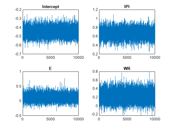
figure;
plot(PosteriorMdl.Sigma2Draws);
title('Sigma2');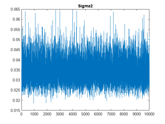
The trace plots indicate that the draws seem to mix well. The plot shows no detectable transience or serial correlation, and the draws do not jump between states.
Plot the posterior distributions of the coefficients and disturbance variance.
figure;
plot(PosteriorMdl)
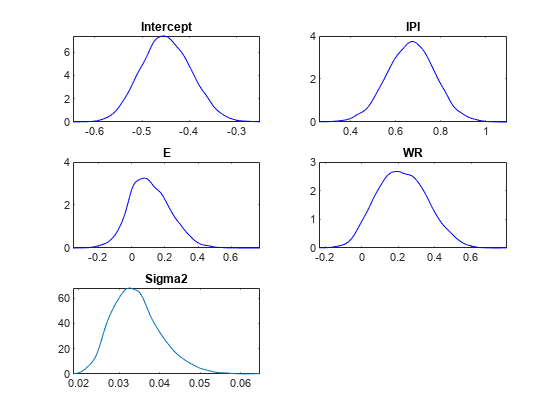
E and WR might not be important predictors because 0 is within the region of high density in their posterior distributions.
Consider the linear regression model in Create Prior Model for Bayesian Lasso Regression and its implementation in Perform Variable Selection Using Default Lasso Shrinkage.
When you implement lasso regression, a common practice is to standardize variables. However, if you want to preserve the interpretation of the coefficients, but the variables have different scales, then you can perform differential shrinkage by specifying a different shrinkage for each coefficient.
Create a prior model for performing Bayesian lasso regression. Specify the number of predictors p and the names of the regression coefficients.
p = 3;
PriorMdl = bayeslm(p,'ModelType','lasso','VarNames',["IPI" "E" "WR"]);
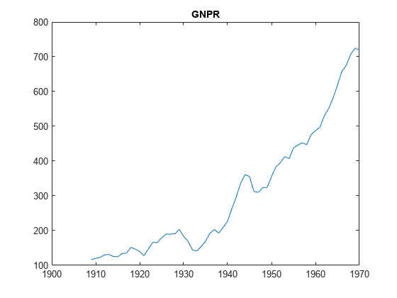
Load the Nelson-Plosser data set. Create variables for the response and predictor series. Determine whether the variables have exponential trends by plotting each in separate figures.
load Data_NelsonPlosser
X = DataTable{:,PriorMdl.VarNames(2:end)};
y = DataTable{:,'GNPR'};

figure;
plot(dates,y)
title('GNPR')
for j = 1:3
    figure;
    plot(dates,X(:,j));
    title(PriorMdl.VarNames(j + 1));
end
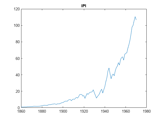
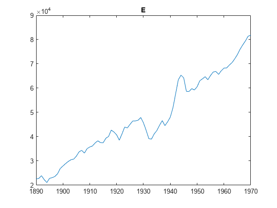
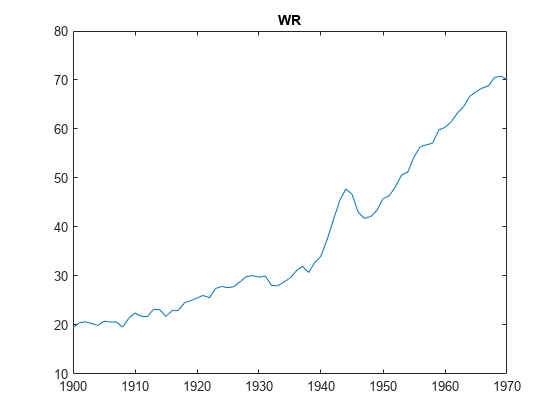
The variables GNPR, IPI, and WR appear to have an exponential trend.
Remove the exponential trend from the variables GNPR, IPI, and WR.
y = log(y);
X(:,[1 3]) = log(X(:,[1 3]));
All predictor variables have different scales (for more details, enter Description at the command line). Display the mean of each predictor. Remove observations containing leading missing values from all predictors.
predmeans = mean(X,'omitnan')predmeans = 1×3
104 ×
0.0002 4.7700 0.0004
The values of the second predictor are much greater than those of the other two predictors and the response. Therefore, the regression coefficient of the second predictor can appear close to zero.
Using dot notation, attribute a very low shrinkage to the intercept, a shrinkage of 0.1 to the first and third predictors, and a shrinkage of 1000 to the second predictor.
PriorMdl.Lambda = [1e-5 0.1 1e4 0.1];
Implement Bayesian lasso regression by estimating the marginal posterior distributions of and . Because Bayesian lasso regression uses MCMC for estimation, set a random number seed to reproduce the results.
rng(1);
PosteriorMdl = estimate(PriorMdl,X,y);
Method: lasso MCMC sampling with 10000 draws
Number of observations: 62
Number of predictors:   4

           |  Mean     Std         CI95        Positive  Distribution
----------------------------------------------------------------------
 Intercept | 2.0281  0.6839  [ 0.679,  3.323]    0.999     Empirical
 IPI       | 0.3534  0.2497  [-0.139,  0.839]    0.923     Empirical
 E         | 0.0000  0.0000  [-0.000,  0.000]    0.762     Empirical
 WR        | 0.5250  0.3482  [-0.126,  1.209]    0.937     Empirical
 Sigma2    | 0.0315  0.0055  [ 0.023,  0.044]    1.000     Empirical
Consider the linear regression model in Create Prior Model for Bayesian Lasso Regression.
Perform Bayesian lasso regression:
Create a Bayesian lasso prior model for the regression coefficients and disturbance variance. Use the default shrinkage.
Hold out the last 10 periods of data from estimation.
Estimate the marginal posterior distributions.
p = 3;
PriorMdl = bayeslm(p,'ModelType','lasso','VarNames',["IPI" "E" "WR"]);

load Data_NelsonPlosser
fhs = 10; % Forecast horizon size
X = DataTable{1:(end - fhs),PriorMdl.VarNames(2:end)};
y = DataTable{1:(end - fhs),'GNPR'};
XF = DataTable{(end - fhs + 1):end,PriorMdl.VarNames(2:end)}; % Future predictor data
yFT = DataTable{(end - fhs + 1):end,'GNPR'};                  % True future responses

rng(1); % For reproducibility
PosteriorMdl = estimate(PriorMdl,X,y,'Display',false);
Forecast responses using the posterior predictive distribution and the future predictor data XF. Plot the true values of the response and the forecasted values.
yF = forecast(PosteriorMdl,XF);

figure;
plot(dates,DataTable.GNPR);
hold on
plot(dates((end - fhs + 1):end),yF)
h = gca;
hp = patch([dates(end - fhs + 1) dates(end) dates(end) dates(end - fhs + 1)],...
    h.YLim([1,1,2,2]),[0.8 0.8 0.8]);
uistack(hp,'bottom');
legend('Forecast Horizon','True GNPR','Forecasted GNPR','Location','NW')
title('Real Gross National Product: 1909 - 1970');
ylabel('rGNP');
xlabel('Year');
hold off
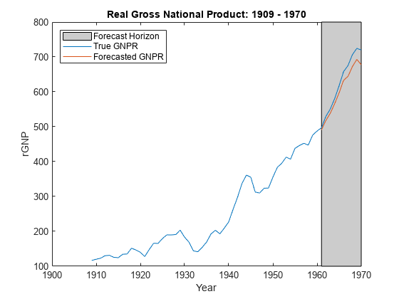
yF is a 10-by-1 vector of future values of real GNP corresponding to the future predictor data.
Estimate the forecast root mean squared error (RMSE).
frmse = sqrt(mean((yF - yFT).^2))
frmse =
25.4831
The forecast RMSE is a relative measure of forecast accuracy. Specifically, you estimate several models using different assumptions. The model with the lowest forecast RMSE is the best-performing model of the ones being compared.
When you perform Bayesian lasso regression, a best practice is to search for appropriate shrinkage values. One way to do so is to estimate the forecast RMSE over a grid of shrinkage values, and choose the shrinkage that minimizes the forecast RMSE.
More About
Tips
Lambdais a tuning parameter. Therefore, perform Bayesian lasso regression using a grid of shrinkage values, and choose the model that best balances a fit criterion and model complexity.For estimation, simulation, and forecasting, MATLAB® does not standardize predictor data. If the variables in the predictor data have different scales, then specify a shrinkage parameter for each predictor by supplying a numeric vector for
Lambda.
Alternative Functionality
The bayeslm function can create any supported prior model object for Bayesian linear regression.
References
[1] Park, T., and G. Casella. "The Bayesian Lasso." Journal of the American Statistical Association. Vol. 103, No. 482, 2008, pp. 681–686.
Version History
Introduced in R2018b