simsmooth
Simulation smoother of Bayesian vector autoregression (VAR) model
Syntax
Description
simsmooth is well suited for advanced applications, such as out-of-sample conditional forecasting from the posterior predictive distribution of a Bayesian VAR(p) model, VARX(p) model forecasting, missing value imputation, and parameter estimation in the presence of missing values. Also, simsmooth enables you to adjust the Gibbs sampler for out-of-sample forecasting. To estimate out-of-sample forecasts from a Bayesian VAR(p) model, see forecast.
[ returns 1000 random draws of coefficient vectors λ
CoeffDraws,SigmaDraws] = simsmooth(PriorMdl,Y)Coeff and innovations covariance matrices Σ Sigma, drawn from the posterior distribution formed by combining the prior Bayesian VAR(p) model
PriorMdl and the response data Y.
The sampling procedure includes a Bayesian data augmentation step that uses the Kalman filter (see Algorithms). During sampling, simsmooth replaces non-presample missing values in Y, indicated by NaN values, with imputed values.
[ uses additional options specified by one or more name-value pair arguments. For example, you can set the number of random draws from the distribution or specify the presample response data.CoeffDraws,SigmaDraws] = simsmooth(PriorMdl,Y,Name,Value)
[ also returns the imputed response values of each draw CoeffDraws,SigmaDraws,NaNDraws]
= simsmooth(___)NaNDraws using any of the input argument combinations in the previous syntaxes.
[ also returns the mean CoeffDraws,SigmaDraws,NaNDraws,YMean,YStd]
= simsmooth(___)YMean and standard deviation YStd of the posterior predictive distribution of the augmented data.
Examples
When simulate estimates the posterior distribution from which to draw parameters, it removes all rows in the data that contain at least one missing value (NaN). However, simsmooth uses Bayesian data augmentation to impute non-presample missing values during posterior estimation.
Consider the 3-D VAR(4) model for the US inflation (INFL), unemployment (UNRATE), and federal funds (FEDFUNDS) rates.
For all , is a series of independent 3-D normal innovations with a mean of 0 and covariance . Assume a weak conjugate prior distribution for the parameters .
Load and Preprocess Data
Load the US macroeconomic data set. Compute the inflation rate, and stabilize the unemployment and federal funds rates.
load Data_USEconModel
seriesnames = ["INFL" "UNRATE" "FEDFUNDS"];
DataTimeTable.INFL = 100*[NaN; price2ret(DataTimeTable.CPIAUCSL)];
DataTimeTable.DUNRATE = [NaN; diff(DataTimeTable.UNRATE)];
DataTimeTable.DFEDFUNDS = [NaN; diff(DataTimeTable.FEDFUNDS)];
seriesnames(2:3) = "D" + seriesnames(2:3);
Several series have leading NaN values because their measurements were not available at the same time as other measurements. Because leading NaN values can interfere with presample specification, remove all rows containing at least one leading missing value.
rmldDataTimeTable = rmmissing(DataTimeTable(:,seriesnames));
Create Prior Model
Create a weak conjugate prior model by specifying large coefficient prior variances. Specify the response series names.
numseries = numel(seriesnames);
numlags = 4;

PriorMdl = conjugatebvarm(numseries,numlags,'SeriesNames',seriesnames);
numcoeffseqn = size(PriorMdl.V,1);
PriorMdl.V = 1e4*eye(numcoeffseqn);
Randomly Place Missing Values in Data
To illustrate simulation in the presence of missing values, randomly place missing values in the data after the presample period.
rng(1)                          % For reproducibility
T = size(rmldDataTimeTable,1);
idxpre = 1:PriorMdl.P;          % Presample period
idxest = (PriorMdl.P + 1):T;    % Estimation period

nmissing = 20;                  % Simulate at most nmissing missing values
sidx = [randsample(idxest,nmissing,true); randsample(1:numseries,nmissing,true)];
lsidx = sub2ind([T,numseries],sidx(1,:),sidx(2,:));
MissData = table2array(rmldDataTimeTable);
MissData(lsidx) = NaN;
MissDataTimeTable = rmldDataTimeTable;
MissDataTimeTable{:,:} = MissData;
Simulate Parameters from Posterior
Draw 1000 parameter sets from the posterior distribution by calling simsmooth, which estimates the posterior distribution of the parameters, and then forms the posterior predictive distribution.
[Coeff,Sigma] = simsmooth(PriorMdl,MissDataTimeTable.Variables);
Coeff is a 39-by-1000 matrix of randomly drawn coefficient vectors from the posterior. Sigma is a 3-by-3-by-1000 array of randomly drawn innovations covariance matrices.
By default, simsmooth initializes the VAR model by using the first four observations in the data.
To associate rows of Coeff to coefficients, obtain a summary of the prior distribution by using summarize. In a table, display the first set of randomly drawn coefficients with corresponding names.
Summary = summarize(PriorMdl,'off');
table(Coeff(:,1),'RowNames',Summary.CoeffMap)
ans=39×1 table
                      Var1
                   __________

    AR{1}(1,1)        0.22109
    AR{1}(1,2)       -0.24034
    AR{1}(1,3)       0.093315
    AR{2}(1,1)        0.18329
    AR{2}(1,2)       -0.23178
    AR{2}(1,3)      -0.026301
    AR{3}(1,1)        0.39991
    AR{3}(1,2)        0.41141
    AR{3}(1,3)       0.054702
    AR{4}(1,1)       0.024944
    AR{4}(1,2)       -0.37372
    AR{4}(1,3)     -0.0095642
    Constant(1)       0.21499
    AR{1}(2,1)      -0.073776
    AR{1}(2,2)        0.36086
    AR{1}(2,3)       0.071088
      ⋮
Alternatively, you can create an empirical model from the draws, and use summarize to display the model by specifying any display option.
Display a summary of the posterior draws as an equation.
EmpMdl = empiricalbvarm(numseries,numlags,'SeriesNames',seriesnames,...
    'CoeffDraws',Coeff,'SigmaDraws',Sigma);
summarize(EmpMdl,'equation')
                                                                                 VAR Equations
           | INFL(-1)  DUNRATE(-1)  DFEDFUNDS(-1)  INFL(-2)  DUNRATE(-2)  DFEDFUNDS(-2)  INFL(-3)  DUNRATE(-3)  DFEDFUNDS(-3)  INFL(-4)  DUNRATE(-4)  DFEDFUNDS(-4)  Constant
------------------------------------------------------------------------------------------------------------------------------------------------------------------------------
 INFL      |  0.1447     -0.3685        0.1013      0.2974     -0.0959        0.0360      0.4115      0.2244        0.0474      0.0265     -0.2321        0.0030      0.1095
           | (0.0744)    (0.1314)      (0.0370)    (0.0833)    (0.1509)      (0.0398)    (0.0833)    (0.1440)      (0.0403)    (0.0879)    (0.1301)      (0.0370)    (0.0744)
 DUNRATE   | -0.0187      0.4445        0.0314      0.0836      0.2372        0.0489     -0.0407     -0.0548       -0.0064      0.0483     -0.1753        0.0027     -0.0597
           | (0.0447)    (0.0808)      (0.0234)    (0.0514)    (0.0863)      (0.0230)    (0.0507)    (0.0906)      (0.0243)    (0.0514)    (0.0779)      (0.0225)    (0.0466)
 DFEDFUNDS | -0.2046     -1.1927       -0.2524      0.2864     -0.2282       -0.2657      0.2709     -0.6231        0.0289     -0.0404      0.1043       -0.1236     -0.2952
           | (0.1530)    (0.2931)      (0.0816)    (0.1832)    (0.3123)      (0.0857)    (0.1736)    (0.3105)      (0.0900)    (0.1866)    (0.2880)      (0.0758)    (0.1684)

       Innovations Covariance Matrix
           |   INFL     DUNRATE  DFEDFUNDS
-------------------------------------------
 INFL      |  0.2842   -0.0098     0.1346
           | (0.0286)  (0.0122)   (0.0464)
 DUNRATE   | -0.0098    0.1062    -0.1496
           | (0.0122)  (0.0106)   (0.0296)
 DFEDFUNDS |  0.1346   -0.1496     1.3187
           | (0.0464)  (0.0296)   (0.1422)
Consider the 3-D VAR(4) model of Simulate Parameters from Posterior Distribution in Presence of Missing Values.
Load the US macroeconomic data set. Compute the inflation rate, and stabilize the unemployment and federal funds rates.
load Data_USEconModel
seriesnames = ["INFL" "UNRATE" "FEDFUNDS"];
DataTimeTable.INFL = 100*[NaN; price2ret(DataTimeTable.CPIAUCSL)];
DataTimeTable.DUNRATE = [NaN; diff(DataTimeTable.UNRATE)];
DataTimeTable.DFEDFUNDS = [NaN; diff(DataTimeTable.FEDFUNDS)];
seriesnames(2:3) = "D" + seriesnames(2:3);
Remove all rows that contain leading missing values.
rmldDataTimeTable = rmmissing(DataTimeTable(:,seriesnames));
Create a weak conjugate prior model. Specify the response series names.
numseries = numel(seriesnames);
numlags = 4;

PriorMdl = conjugatebvarm(numseries,numlags,'SeriesNames',seriesnames);
numcoeffseqn = size(PriorMdl.V,1);
PriorMdl.V = 1e4*eye(numcoeffseqn);
Randomly place missing values in the data after the presample period.
rng(1)                          % For reproducibility
T = size(rmldDataTimeTable,1);
idxpre = 1:PriorMdl.P;          % Presample period
idxest = (PriorMdl.P + 1):T;    % Estimation period

nmissing = 20;                  % Simulate at most nmissing missing values
sidx = [randsample(idxest,nmissing,true); randsample(1:numseries,nmissing,true)];
lsidx = sub2ind([T,numseries],sidx(1,:),sidx(2,:));
MissData = table2array(rmldDataTimeTable);
MissData(lsidx) = NaN;
MissDataTimeTable = rmldDataTimeTable;
MissDataTimeTable{:,:} = MissData;
Draw 1000 parameter sets from the posterior distribution by calling simsmooth. Return the values that the simulation smoother imputes for the missing observations.
[~,~,NaNDraws] = simsmooth(PriorMdl,MissDataTimeTable.Variables);
NaNDraws is a 19-by-1000 matrix of randomly drawn response vectors from the posterior predictive distribution. Elements correspond to the missing values in the data ordered by a column-wise search. For example, NaNDraws(3,1) is the first randomly drawn imputed response of the third missing value in the data. Find the corresponding value in the data.
[idxi,idxj] = find(ismissing(MissDataTimeTable),3);
responsename = seriesnames(idxj(end))
responsename =
"INFL"
observationtime = MissDataTimeTable.Time(idxi(end))
observationtime = datetime
   Q3-65
Plot the empirical distribution of the imputed values of the inflation rate during Q3-65.
histogram(NaNDraws(3,:))
title('Q3-65 Inflation Rate Empirical Distribution')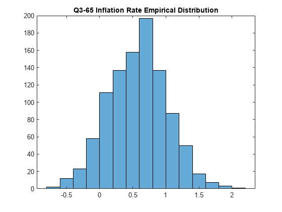
Consider the 3-D VAR(4) model of Simulate Parameters from Posterior Distribution in Presence of Missing Values.
Load the US macroeconomic data set. Compute the inflation rate, stabilize the unemployment and federal funds rates, and remove missing values (the data includes leading missing values only).
load Data_USEconModel
seriesnames = ["INFL" "UNRATE" "FEDFUNDS"];
DataTimeTable.INFL = 100*[NaN; price2ret(DataTimeTable.CPIAUCSL)];
DataTimeTable.DUNRATE = [NaN; diff(DataTimeTable.UNRATE)];
DataTimeTable.DFEDFUNDS = [NaN; diff(DataTimeTable.FEDFUNDS)];
seriesnames(2:3) = "D" + seriesnames(2:3);
rmDataTimeTable = rmmissing(DataTimeTable);
Create a weak conjugate prior model. Specify the response series names.
numseries = numel(seriesnames);
numlags = 4;

PriorMdl = conjugatebvarm(numseries,numlags,'SeriesNames',seriesnames);
numcoeffseqn = size(PriorMdl.V,1);
PriorMdl.V = 1e4*eye(numcoeffseqn);
Simulate 5000 coefficients and innovations covariance matrices from the posterior distribution. Specify a burn-in period of 1000 and a thinning factor of 5.
rng(1); % For reproducibility
[Coeff,Sigma] = simsmooth(PriorMdl,rmDataTimeTable{:,seriesnames},...
    'NumDraws',5000,'BurnIn',1000,'Thin',5);
Coeff is a 39-by-5000 matrix of coefficients, and Sigma is a 3-by-3-by-5000 array of innovations covariance matrices. Both Coeff and Sigma are randomly drawn from the posterior distribution.
Consider the 3-D VAR(4) model of Simulate Parameters from Posterior Distribution in Presence of Missing Values. In this case, assume that the prior model is semiconjugate.
Load the US macroeconomic data set. Compute the inflation rate, stabilize the unemployment and federal funds rates, and remove missing values (the data includes leading missing values only).
load Data_USEconModel
seriesnames = ["INFL" "UNRATE" "FEDFUNDS"];
DataTimeTable.INFL = 100*[NaN; price2ret(DataTimeTable.CPIAUCSL)];
DataTimeTable.DUNRATE = [NaN; diff(DataTimeTable.UNRATE)];
DataTimeTable.DFEDFUNDS = [NaN; diff(DataTimeTable.FEDFUNDS)];
seriesnames(2:3) = "D" + seriesnames(2:3);
rmDataTimeTable = rmmissing(DataTimeTable);
Create a semiconjugate prior model. Specify the response series names.
numseries = numel(seriesnames);
numlags = 4;

PriorMdl = bayesvarm(numseries,numlags,'ModelType','semiconjugate',...
    'SeriesNames',seriesnames);
To obtain starting values for the coefficients, consider the coefficients from a VAR model fitted to the first 30 observations.
Define index sets that partition the data into four sets:
Length p = 4 initialization period for the dynamic component of the model
= 30 observations to estimate the VAR for the coefficient initial values
Length p = 4 initialization period for the dynamic component of the Bayesian VAR model
Remaining observations to estimate the posterior
T = height(rmDataTimeTable);
n0 = 30;
idxpre0 = 1:PriorMdl.P;
idxest0 = (idxpre0(end) + 1):(idxpre0(end) + 1 + n0);
idxpre1 = (idxest0(end) + 1 - PriorMdl.P):idxest0(end);
idxest1 = (idxest0(end) + 1):T;
n1 = numel(idxest1);
Obtain initial coefficient values by fitting a VAR model to the first 34 observations. Use the first four observations as a presample.
Mdl0 = varm(PriorMdl.NumSeries,PriorMdl.P);
EstMdl0 = estimate(Mdl0,rmDataTimeTable{idxest0,seriesnames},'Y0',rmDataTimeTable{idxpre0,seriesnames});
estimate returns a model object containing the AR coefficient estimates in matrix form and the constants in a vector. The Bayesian VAR functions require initial coefficient values in a vector. Format the initial coefficient values.
Coeff0 = [EstMdl0.AR{:} EstMdl0.Constant].';
Coeff0 = Coeff0(:);
Simulate 1000 coefficients and innovations covariance matrices from the posterior distribution. Specify the remaining observations from which to estimate the posterior. Initialize the VAR model by specifying the last four observations in the previous estimation sample as a presample, and specify the initial coefficient vector to initialize the posterior sample.
rng(1) % For reproducibility
[Coeff,Sigma] = simsmooth(PriorMdl,rmDataTimeTable{idxest1,seriesnames},...
    'Y0',rmDataTimeTable{idxpre1,seriesnames},'Coeff0',Coeff0);
Coeff is a 39-by-1000 matrix of coefficients and Sigma is a 3-by-3-by-1000 array of innovations covariance matrices. Both Coeff and Sigma are randomly drawn from the posterior distribution.
Consider the 3-D VAR(4) model of Simulate Parameters from Posterior Distribution in Presence of Missing Values.
Load and Preprocess Data
Load the US macroeconomic data set. Compute the inflation rate, stabilize the unemployment and federal funds rates, and remove missing values (the data includes leading missing values only).
load Data_USEconModel
seriesnames = ["INFL" "UNRATE" "FEDFUNDS"];
DataTimeTable.INFL = 100*[NaN; price2ret(DataTimeTable.CPIAUCSL)];
DataTimeTable.DUNRATE = [NaN; diff(DataTimeTable.UNRATE)];
DataTimeTable.DFEDFUNDS = [NaN; diff(DataTimeTable.FEDFUNDS)];
seriesnames(2:3) = "D" + seriesnames(2:3);
rmDataTimeTable = rmmissing(DataTimeTable);
Create Prior Model
Create a weak conjugate prior model. Specify the response series names.
numseries = numel(seriesnames);
numlags = 4;

PriorMdl = conjugatebvarm(numseries,numlags,'SeriesNames',seriesnames);
numcoeffseqn = size(PriorMdl.V,1);
PriorMdl.V = 1e4*eye(numcoeffseqn);
Forecast Responses Using forecast
Directly forecast two years (eight quarters) of observations from the posterior predictive distribution. forecast estimates the posterior distribution of the parameters, and then forms the posterior predictive distribution.
rng(1); % For reproducibility
numperiods = 8;
YF = forecast(PriorMdl,numperiods,rmDataTimeTable{:,seriesnames});
YF is an 8-by-3 matrix of forecasted responses.
Plot the forecasted responses.
fh = rmDataTimeTable.Time(end) + calquarters(1:8);
for j = 1:PriorMdl.NumSeries
    subplot(3,1,j)
    plot(rmDataTimeTable.Time(end - 20:end),rmDataTimeTable{end - 20:end,seriesnames(j)},'r',...
        [rmDataTimeTable.Time(end) fh],[rmDataTimeTable{end,seriesnames(j)}; YF(:,j)],'b');
    legend("Observed","Forecasted",'Location','NorthWest')
    title(seriesnames(j))
end
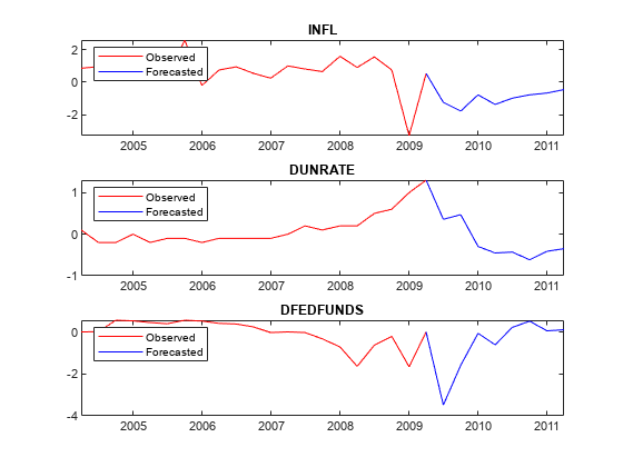
Forecast Responses Using simsmooth
Configure the data set for obtaining forecasts from simsmooth by concatenating a numperiods-by-numseries timetable of missing values to the end of the set.
fTT = array2timetable(NaN(numperiods,numseries),'RowTimes',fh,...
    'VariableNames',seriesnames);
frmDataTimeTable = [rmDataTimeTable(:,seriesnames); fTT];
tail(frmDataTimeTable)
    Time     INFL    DUNRATE    DFEDFUNDS
    _____    ____    _______    _________

    Q2-09    NaN       NaN         NaN
    Q3-09    NaN       NaN         NaN
    Q4-09    NaN       NaN         NaN
    Q1-10    NaN       NaN         NaN
    Q2-10    NaN       NaN         NaN
    Q3-10    NaN       NaN         NaN
    Q4-10    NaN       NaN         NaN
    Q1-11    NaN       NaN         NaN
Forecast the VAR model using simsmooth. Like forecast, simsmooth estimates the posterior distribution, so it requires a prior model and data. Specify the data containing the trailing NaNs.
[~,~,~,YMean] = simsmooth(PriorMdl,frmDataTimeTable.Variables);
YMean is almost equal to frmDataTimeTable, with these exceptions:
YMeanexcludes rows corresponding to the presample periodfrmDataTimeTable(1:4,:).If
frmDataTimeTable(j,k)isNaN,YMean(j,k)is the mean of the posterior predictive distribution of responsekat timej.
Create a timetable from YMean.
YMeanTT = array2timetable(YMean,'RowTimes',frmDataTimeTable.Time((PriorMdl.P + 1):end),...
    'VariableNames',seriesnames);
Plot the forecasted responses.
tiledlayout(3,1)
for j = 1:PriorMdl.NumSeries
    nexttile
    plot(YMeanTT.Time((end - 20 - numperiods):(end - numperiods)),YMeanTT{(end - 20 - numperiods):(end - numperiods),j},'r',...
        YMeanTT.Time((end - numperiods):end),YMeanTT{(end - numperiods):end,j},'b');
        legend("Observed","Forecasted",'Location','NorthWest')
    title(seriesnames(j))
end
Consider the 3-D VAR(4) model of Simulate Parameters from Posterior Distribution in Presence of Missing Values.
Load the US macroeconomic data set. Compute the inflation rate, stabilize the unemployment and federal funds rates, and remove missing values (the data includes leading missing values only).
load Data_USEconModel
seriesnames = ["INFL" "UNRATE" "FEDFUNDS"];
DataTimeTable.INFL = 100*[NaN; price2ret(DataTimeTable.CPIAUCSL)];
DataTimeTable.DUNRATE = [NaN; diff(DataTimeTable.UNRATE)];
DataTimeTable.DFEDFUNDS = [NaN; diff(DataTimeTable.FEDFUNDS)];
seriesnames(2:3) = "D" + seriesnames(2:3);
rmDataTimeTable = rmmissing(DataTimeTable);
Create a weak conjugate prior model. Specify the response series names.
numseries = numel(seriesnames);
numlags = 4;
PriorMdl = conjugatebvarm(numseries,numlags,'SeriesNames',seriesnames);
numcoeffseqn = size(PriorMdl.V,1);
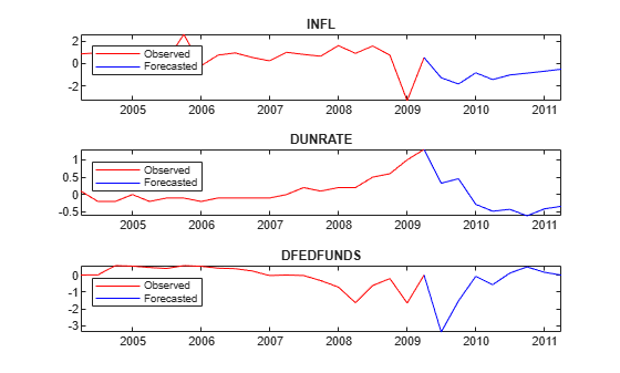
PriorMdl.V = 1e4*eye(numcoeffseqn);Conditional forecasting occurs when response values are known or hypothesized in the forecast horizon, and unknown values are forecasted conditioned on the known values. Suppose that the unemployment rate change (DUNRATE) remains at one percentage point through a two-year forecast horizon.
Configure the data set for obtaining forecasts from simsmooth by concatenating a numperiods-by-numseries timetable of missing values to the end of the set. For the unemployment rate change, replace the missing values with a vector of ones.
rng(1); % For reproducibility
numperiods = 8;
fh = rmDataTimeTable.Time(end) + calquarters(1:8);

fTT = array2timetable(NaN(numperiods,numseries),'RowTimes',fh,...
    'VariableNames',seriesnames);

frmDataTimeTable = [rmDataTimeTable(:,seriesnames); fTT];
frmDataTimeTable.DUNRATE((end - numperiods + 1):end) = ones(numperiods,1);
tail(frmDataTimeTable)
    Time     INFL    DUNRATE    DFEDFUNDS
    _____    ____    _______    _________

    Q2-09    NaN        1          NaN
    Q3-09    NaN        1          NaN
    Q4-09    NaN        1          NaN
    Q1-10    NaN        1          NaN
    Q2-10    NaN        1          NaN
    Q3-10    NaN        1          NaN
    Q4-10    NaN        1          NaN
    Q1-11    NaN        1          NaN
Obtain forecasts for the inflation rate and federal funds rate change series, given that the unemployment rate change is one for the entire horizon.
[~,~,~,YMean] = simsmooth(PriorMdl,frmDataTimeTable.Variables);
YMean is almost equal to frmDataTimeTable, with these exceptions:
YMeanexcludes rows corresponding to the presample periodfrmDataTimeTable(1:4,:).If
frmDataTimeTable(j,k)isNaN,YMean(j,k)is the mean of the posterior predictive distribution of responsekat timej.
Create a timetable from YMean.
YMeanTT = array2timetable(YMean,'RowTimes',frmDataTimeTable.Time((PriorMdl.P + 1):end),...
    'VariableNames',seriesnames);
Plot the forecasted responses.
for j = 1:PriorMdl.NumSeries
    subplot(3,1,j)
    plot(YMeanTT.Time((end - 20 - numperiods):(end - numperiods)),YMeanTT{(end - 20 - numperiods):(end - numperiods),j},'r',...
        YMeanTT.Time((end - numperiods):end),YMeanTT{(end - numperiods):end,j},'b');
        legend("Observed","Forecasted",'Location','NorthWest')
    title(seriesnames(j))
end
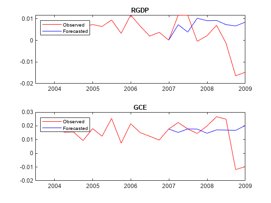
Consider the 2-D VARX(1) model for the US real GDP (RGDP) and investment (GCE) rates that treats the personal consumption (PCEC) rate as exogenous:
For all , is a series of independent 2-D normal innovations with a mean of 0 and covariance . Assume the following prior distributions:
, where M is a 4-by-2 matrix of means and is the 4-by-4 among-coefficient scale matrix. Equivalently, .
where Ω is the 2-by-2 scale matrix and is the degrees of freedom.
Load the US macroeconomic data set. Compute the real GDP, investment, and personal consumption rate series. Remove all missing values from the resulting series.
load Data_USEconModel
DataTimeTable.RGDP = DataTimeTable.GDP./DataTimeTable.GDPDEF;
seriesnames = ["PCEC"; "RGDP"; "GCE"];
rates = varfun(@price2ret,DataTimeTable,'InputVariables',seriesnames);
rates = rmmissing(rates);
rates.Properties.VariableNames = seriesnames;
Create a conjugate prior model for the 2-D VARX(1) model parameters.
numseries = 2;
numlags = 1;
numpredictors = 1;
PriorMdl = conjugatebvarm(numseries,numlags,'NumPredictors',numpredictors,...
    'SeriesNames',seriesnames(2:end));
Create index sets that partition the data into estimation and forecast samples. Specify a forecast horizon of two years.
T = size(rates,1);
numperiods = 8;
idxest = 1:(T - numperiods); % Includes presample
idxf = (T - numperiods + 1):T;
idxtot = [idxest idxf];
The simulation smoother forecasts by imputing missing values. Therefore, create a data set that contains missing values for the responses in the forecast horizon.
missingrates = rates;
missingrates{idxf,PriorMdl.SeriesNames} = nan(numperiods,PriorMdl.NumSeries);
Forecast responses in the forecast horizon. Specify presample observations and the exogenous predictor data. Return standard deviations of the posterior predictive distribution.
rng(1) % For reproducibility
[~,~,~,YMean,YStd] = simsmooth(PriorMdl,missingrates{:,PriorMdl.SeriesNames},...
    'X',missingrates{:,seriesnames(1)});
Create a timetable from YMean.
YMeanTT = array2timetable(YMean,'RowTimes',rates.Time((PriorMdl.P + 1):end),...
    'VariableNames',PriorMdl.SeriesNames);
Plot the forecasted responses.
tiledlayout(2,1)
for j = 1:PriorMdl.NumSeries
    nexttile
    plot(rates.Time((end - 20):end),rates{(end - 20):end,PriorMdl.SeriesNames(j)},'r',...
        YMeanTT.Time((end - numperiods):end),YMeanTT{(end - numperiods):end,PriorMdl.SeriesNames(j)},'b');
        legend("Observed","Forecasted",'Location','NorthWest')
    title(PriorMdl.SeriesNames(j))
end
Input Arguments
Name-Value Arguments
Output Arguments
More About
Tips
Monte Carlo simulation is subject to variation. If
simsmoothuses Monte Carlo simulation, then estimates and inferences might vary when you callsimsmoothmultiple times under seemingly equivalent conditions. To reproduce estimation results, set a random number seed by usingrngbefore callingsimsmooth.
Algorithms
This figure shows how
simsmoothreduces the sample by using the values ofNumDraws,Thin, andBurnIn. Rectangles represent successive draws from the distribution.simsmoothremoves the white rectangles from the sample. The remainingNumDrawsblack rectangles compose the sample.
simsmoothdoes not return default starting values that it generates.
References
[1] Litterman, Robert B. "Forecasting with Bayesian Vector Autoregressions: Five Years of Experience." Journal of Business and Economic Statistics 4, no. 1 (January 1986): 25–38. https://doi.org/10.2307/1391384.
Version History
Introduced in R2020a