Main Content

collintest

Belsley collinearity diagnostics

Description

[sValue,condIdx,VarDecomp] = collintest(X) displays, at the command window, Belsley collinearity diagnostics for assessing the strength and sources of collinearity among variables in the input matrix of time series data. The function also returns the singular values in decreasing order, condition indices, and variance decomposition proportions.

example

VarDecompTbl = collintest(Tbl) displays the Belsley collinearity diagnostics on all the variables of the input table or timetable. The function also returns a table containing variables for the singular values and condition indices, and variables for the variance-decomposition proportions associated with each time series.

To select a subset of variables, for which to compute collinearity diagnostics, use the DataVariables name-value argument.

example

[___] = collintest(___,Name=Value) specifies options using one or more name-value arguments in addition to any of the input argument combinations in previous syntaxes. collintest returns the output argument combination for the corresponding input arguments. For example, collintest(Tbl,Plot="on",Display="off",DataVariables=1:5) plots the Belslely collinearity diagnostics for the first 5 variables of the table Tbl to a figure instead of the command window.

example

collintest(ax,Plot="on",___) plots on the axes specified by ax instead of the current axes (gca). ax can precede any of the input argument combinations in the previous syntaxes.

[___,h] = collintest(___,Plot="on") plots the diagnostics of the input series and additionally returns handles to plotted graphics objects h. Use elements of h to modify properties of the plot after you create it.

Examples

collapse all

Display collinearity diagnostics for multiple time series using the default options of collintest. Input the time series data as a numeric matrix.

Load data of Canadian inflation and interest rates Data_Canada.mat, which contains the series in the matrix Data.

load Data_Canada

Display the Belsley collinearity diagnostics at the command window. Return the singular values, condition indices, and variance decomposition proportions.

series'
ans = 5x1 cell
    {'(INF_C) Inflation rate (CPI-based)'         }
    {'(INF_G) Inflation rate (GDP deflator-based)'}
    {'(INT_S) Interest rate (short-term)'         }
    {'(INT_M) Interest rate (medium-term)'        }
    {'(INT_L) Interest rate (long-term)'          }

[sValue,condIdx,VarDecomp] = collintest(Data);
Variance Decomposition

 sValue  condIdx   Var1    Var2    Var3    Var4    Var5  
---------------------------------------------------------
 2.1748    1      0.0012  0.0018  0.0003  0.0000  0.0001 
 0.4789   4.5413  0.0261  0.0806  0.0035  0.0006  0.0012 
 0.1602  13.5795  0.3386  0.3802  0.0811  0.0011  0.0137 
 0.1211  17.9617  0.6138  0.5276  0.1918  0.0004  0.0193 
 0.0248  87.8245  0.0202  0.0099  0.7233  0.9979  0.9658 

Only the last row in the display has a condition index larger than the default tolerance, 30. In this row, the last three variables (in the last three columns) have variance-decomposition proportions exceeding the default tolerance, 0.5. These results suggest that the short-, medium-, and long-term interest rates exhibit multicollinearity.

collintest organizes the outputs in the display table.

sValue
sValue = 5×1

    2.1748
    0.4789
    0.1602
    0.1211
    0.0248

condIdx
condIdx = 5×1

    1.0000
    4.5413
   13.5795
   17.9617
   87.8245

VarDecomp
VarDecomp = 5×5

    0.0012    0.0018    0.0003    0.0000    0.0001
    0.0261    0.0806    0.0035    0.0006    0.0012
    0.3386    0.3802    0.0811    0.0011    0.0137
    0.6138    0.5276    0.1918    0.0004    0.0193
    0.0202    0.0099    0.7233    0.9979    0.9658

Display and return collinearity diagnostics for multiple time series, which are variables in a table, using default options.

Load data of Canadian inflation and interest rates Data_Canada.mat. Convert the table DataTable to a timetable.

load Data_Canada
dates = datetime(dates,ConvertFrom="datenum");
TT = table2timetable(DataTable,RowTimes=dates);
TT.Observations = [];

Display the Belsley collinearity diagnostics, using all default options.

VarDecompTbl = collintest(TT)
Variance Decomposition

 sValue  condIdx   INF_C   INF_G   INT_S   INT_M   INT_L 
---------------------------------------------------------
 2.1748    1      0.0012  0.0018  0.0003  0.0000  0.0001 
 0.4789   4.5413  0.0261  0.0806  0.0035  0.0006  0.0012 
 0.1602  13.5795  0.3386  0.3802  0.0811  0.0011  0.0137 
 0.1211  17.9617  0.6138  0.5276  0.1918  0.0004  0.0193 
 0.0248  87.8245  0.0202  0.0099  0.7233  0.9979  0.9658 
VarDecompTbl=5×7 table
     sValue     condIdx      INF_C        INF_G        INT_S         INT_M         INT_L   
    ________    _______    _________    _________    __________    __________    __________

      2.1748         1     0.0012446    0.0017784    0.00033202    4.2326e-05    8.0328e-05
     0.47889    4.5413        0.0261     0.080594     0.0034869    0.00057749      0.001159
     0.16015    13.579       0.33864      0.38021      0.081126     0.0011166      0.013662
     0.12108    17.962       0.61384      0.52756       0.19176    0.00035545      0.019308
    0.024763    87.825      0.020173    0.0098575       0.72329       0.99791       0.96579

collintest returns collinearity diagnostics in the table VarDecompTbl, where variables correspond to the singular values, condition indices, and variance-decomposition proportions of each variable in the data (sValue, condIdx, and VarDecomp). The command window display and output table have a similar form.

By default, collintest computes collinearity diagnostics for all variables in the input table. To select a subset of variables from an input table, set the DataVariables option.

Extract the variance-decomposition proportions from the output table.

varnames = DataTable.Properties.VariableNames;
VarDecomp = VarDecompTbl(:,varnames)
VarDecomp=5×5 table
      INF_C        INF_G        INT_S         INT_M         INT_L   
    _________    _________    __________    __________    __________

    0.0012446    0.0017784    0.00033202    4.2326e-05    8.0328e-05
       0.0261     0.080594     0.0034869    0.00057749      0.001159
      0.33864      0.38021      0.081126     0.0011166      0.013662
      0.61384      0.52756       0.19176    0.00035545      0.019308
     0.020173    0.0098575       0.72329       0.99791       0.96579

Plot collinearity diagnostics for all time series in a table.

Load data of Canadian inflation and interest rates Data_Canada.mat.

load Data_Canada

Plot the Belsley collinearity diagnostics for all series.

collintest(DataTable,Plot="on");
Variance Decomposition

 sValue  condIdx   INF_C   INF_G   INT_S   INT_M   INT_L 
---------------------------------------------------------
 2.1748    1      0.0012  0.0018  0.0003  0.0000  0.0001 
 0.4789   4.5413  0.0261  0.0806  0.0035  0.0006  0.0012 
 0.1602  13.5795  0.3386  0.3802  0.0811  0.0011  0.0137 
 0.1211  17.9617  0.6138  0.5276  0.1918  0.0004  0.0193 
 0.0248  87.8245  0.0202  0.0099  0.7233  0.9979  0.9658 

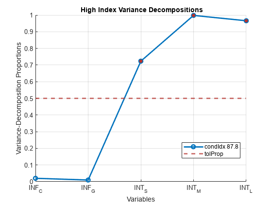
Figure contains an axes object. The axes object with title blank High blank Index blank Variance blank Decompositions, xlabel Variables, ylabel Variance-Decomposition Proportions contains 3 objects of type line, constantline. One or more of the lines displays its values using only markers These objects represent condIdx 87.8, tolProp.

The plot corresponds to the values in the last row of the variance-decomposition proportions, which are the only proportions with a condition index larger than the default tolerance of 30. The interest rate series have variance-decomposition proportions exceeding the default tolerance of 0.5 (red markers in the plot).

Compute collinearity diagnostics for selected time series and an intercept.

Load the credit default data set Data_CreditDefaults.mat. The table DataTable contains the default rate of investment-grade corporate bonds series (IGD, the response variable) and several predictor variables.

load Data_CreditDefaults

Consider a multiple regression model for the default rate that includes an intercept term.

Include a variable in the table of data that represents the intercept in the design matrix (that is, a column of ones). Place the intercept variable at the beginning of the table.

Const = ones(height(DataTable),1);
DataTable = addvars(DataTable,Const,Before=1);

Create a variable that contains all predictor variable names.

varnames = DataTable.Properties.VariableNames;
prednames = varnames(varnames ~= "IGD");

Graph a correlation plot of all predictor variables except for the intercept dummy variable.

figure
corrplot(DataTable,DataVariables=prednames(2:end), ...
    TestR="on");

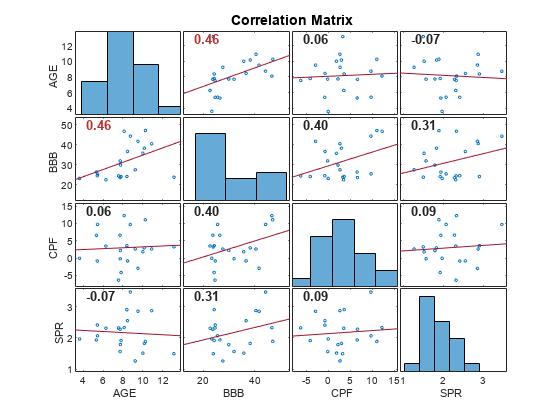
MATLAB figure

The predictor BBB is moderately linearly associated with the other predictors, while all other predictors appear unassociated with each other.

Plot the Belsley collinearity diagnostics of the predictor variables. Adjust the following options for the collinearity diagnostics:

  • Set the condition index tolerance to 10.

  • Set the variance-decomposition proportion tolerance to 0.5.

figure
collintest(DataTable,Plot="on",DataVariables=prednames, ...
    TolIdx=10,TolProp=0.5);
Variance Decomposition

 sValue  condIdx   Const    AGE     BBB     CPF     SPR  
---------------------------------------------------------
 2.0605    1      0.0015  0.0024  0.0020  0.0140  0.0025 
 0.8008   2.5730  0.0016  0.0025  0.0004  0.8220  0.0023 
 0.2563   8.0400  0.0037  0.3208  0.0105  0.0004  0.3781 
 0.1710  12.0464  0.2596  0.0950  0.8287  0.1463  0.0001 
 0.1343  15.3405  0.7335  0.5793  0.1585  0.0173  0.6170 

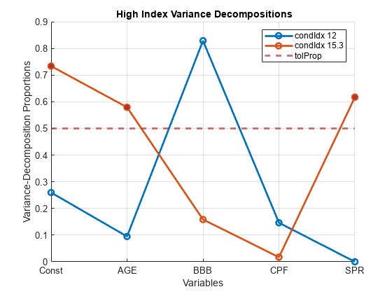
Figure contains an axes object. The axes object with title blank High blank Index blank Variance blank Decompositions, xlabel Variables, ylabel Variance-Decomposition Proportions contains 4 objects of type line, constantline. One or more of the lines displays its values using only markers These objects represent condIdx 12, condIdx 15.3, tolProp.

The row associated with condition index 12 (row 4) has one predictor (BBB) with a proportion above the tolerance 0.5, but collinearity requires two or more predictors for a dependency.

The row associated with condition index 15.3 (row 5) shows a weak dependence involving AGE, SPR, and the intercept, which the correlation plot does not expose.

Input Arguments

collapse all

Time series data, specified as a numObs-by-numVars numeric matrix. Each column of X corresponds to a variable, and each row corresponds to an observation.

Data Types: double

Time series data, specified as a table or timetable with numObs rows. Each row of Tbl is an observation.

Specify numVars variables to include in the diagnostics computations by using the DataVariables argument. The selected variables must be numeric.

Axes on which to plot, specified as an Axes object.

By default, collintest plots to the current axes (gca).

Note

  • To specify a model containing an intercept, include a variable (column) of ones in the time series data.

  • collintest scales all variables to unit length before computing diagnostics; do not center the variables in the data.

  • Impute or remove all missing observations (indicated by NaN entries) in the input data before passing the set to collintest.

Name-Value Arguments

Specify optional pairs of arguments as Name1=Value1,...,NameN=ValueN, where Name is the argument name and Value is the corresponding value. Name-value arguments must appear after other arguments, but the order of the pairs does not matter.

Before R2021a, use commas to separate each name and value, and enclose Name in quotes.

Example: collintest(Tbl,Plot="on",Display="off",DataVariables=1:5) plots the Belslely collinearity diagnostics for the first 5 variables of the table Tbl to a figure instead of the command window.

Unique variable names used in displays and plots of the results, specified as a string vector or cell vector of strings of a length numVars. VarNames(j) specifies the name to use for variable X(:,j) or DataVariables(j).

If an intercept term is present, VarNames must include the intercept term (e.g., include the name "Const").

The software truncates all variable names to the first five characters.

  • If the input time series data is a matrix X, the default is {'var1','var2',...}.

  • If the input time series data is a table or timetable Tbl, the default is Tbl.Properties.VariableNames.

Example: VarNames=["Const" "AGE" "BBD"]

Data Types: char | cell | string

Flag for a command window display of results, specified as a value in this table.

ValueDescription
"on"collintest displays all outputs in tabular form to the command window.
"off"collintest does not display the results to the command window.

Example: Display="off"

Data Types: char | string

Flag for plotting results to a figure, specified as a value in this table.

ValueDescription
"on"

collintest plots critical rows of the output VarDecomp, specifically, rows with condition indices above the input tolerance TolIdx.

If a group of at least two variables in a critical row have variance-decomposition proportions above the input tolerance TolProp, the group is identified with red markers.

"off"collintest does not plot results to a figure.

Example: Plot="on"

Data Types: char | string

Condition index tolerance, specified as a scalar value of at least 1.

collintest uses TolIdx to decide which indices are large enough to infer a near dependency in the data. TolIdx is used only when the Plot argument is "on".

Example: TolIdx=25

Data Types: double

Variance-decomposition proportion tolerance, specified as a numeric scalar in the interval [0,1].

collintest uses TolProp to decide which variables are involved in any near dependency. TolProp is used only when the Plot argument is "on".

Example: TolProp=0.4

Data Types: double

Variables in Tbl for which collintest computes Belsley collinearity diagnostics, specified as a string vector or cell vector of character vectors containing variable names in Tbl.Properties.VariableNames, or an integer or logical vector representing the indices of names. The selected variables must be numeric.

Example: DataVariables=["GDP" "CPI"]

Example: DataVariables=[true true false false] or DataVariables=[1 2] selects the first and second table variables.

Data Types: double | logical | char | cell | string

Output Arguments

collapse all

Singular values of the scaled design matrix composed of the specified time series variables, returned as a numeric vector with elements in descending order. collintest returns sValue when you supply the input X.

Condition indices, returned as a numeric vector with elements in ascending order.

All condition indices have value between 1 and the condition number of the scaled design matrix of the specified time series variables. collintest returns condIdx when you supply the input X.

Large indices identify near dependencies among the specified variables. The size of the indices is a measure of how near dependencies are to collinearity.

Variance-decomposition proportions, returned as a numVars-by-numVars numeric matrix.

Large proportions, combined with a large condition index, identify groups of variables involved in near dependencies. collintest returns VarDecomp when you supply the input X.

The size of the proportions is a measure of how badly the regression is degraded by the dependency.

Collinearity diagnostics summary, returned as a table with variables for the outputs sValue, condIdx, and VarDecomp. collintest returns Tbl when you supply the input Tbl. The value of the VarNames argument determines the variable names of the columns of VarDecomp.

Handles to plotted graphics objects, returned as a graphics array. h contains unique plot identifiers, which you can use to query or modify properties of the plot.

collintest plots only when you set Plot="on".

More About

collapse all

Belsley Collinearity Diagnostics

Belsley collinearity diagnostics assess the strength and sources of collinearity among variables in a multiple linear regression model.

To assess collinearity, the software computes singular values of the scaled variable matrix, X, and then converts them to condition indices. The conditional indices identify the number and strength of any near dependencies between variables in the variable matrix. The software decomposes the variance of the ordinary least squares (OLS) estimates of the regression coefficients in terms of the singular values to identify variables involved in each near dependency, and the extent to which the dependencies degrade the regression.

Condition Indices

The condition indices (condIdx) for a scaled matrix X identify the number and strength of any near dependencies in X.

For scaled matrix X with p columns and singular values (sValue) S1S2Sp, the condition indices of the columns of X are S1/Sj (sValue(1)/sValue(j)), where j = 1,...,p.

All condition indices are bounded between one and the condition number.

Condition Number

The condition number of a scaled matrix X is an overall diagnostic for detecting collinearity.

For scaled matrix X with p columns and singular values (sValue) S1S2Sp, the condition number is S1/Sp (sValue(1)/sValue(end)).

The condition number achieves its lower bound of one when the columns of scaled X are orthonormal. The condition number rises as variates exhibit greater dependency.

A limitation of the condition number as a diagnostic is that it fails to provide specifics on the strength and sources of any near dependencies.

Multiple Linear Regression Model

A multiple linear regression model is a model of the form Y=Xβ+ε. X is a design matrix of regression variables, and β is a vector of regression coefficients.

Singular Values

The singular values (sValue) of a scaled matrix X are the diagonal elements of the matrix S in the singular value decomposition USV.

In descending order, the singular values of the scaled matrix X with p columns are S1S2Sp.

Variance-Decomposition Proportions

Variance-decomposition proportions identify groups of variates involved in near dependencies, and the extent to which the dependencies degrade the regression.

From the singular value decomposition USV of scaled design matrix X (with p columns), define the following quantities:

  • V is the matrix of orthonormal eigenvectors of XX.

  • The singular values (sValue) S1S2Sp are the ordered diagonal elements of the matrix S.

The variance of the OLS estimate of multiple linear regression coefficient i, βi, is proportional to the sum

V(i,1)2/S12+V(i,2)2/S22++V(i,p)2/Sp2,

where V(i,j) denotes element (i,j) of V.

Variance-decomposition proportion (i,j) (VarDecomp) is the proportion of term j in the sum relative to the entire sum, j = 1,...,p.

The terms Sj2 are the eigenvalues of scaled XX. Thus, large variance-decomposition proportions correspond to small eigenvalues of XX, a common diagnostic for collinearity. The singular value decomposition provides a more direct, numerically stable view of the eigensystem of scaled XX.

Tips

  • For purposes of collinearity diagnostics, Belsley [1] shows that column scaling of the design matrix composed of the input time series data is always desirable. However, he also shows that centering the data in X is undesirable. For models with an intercept, if you center the data in X, the role of the constant term in any near dependency is hidden, and yields misleading diagnostics.

  • Tolerances for identifying large condition indices and variance-decomposition proportions are comparable to critical values in standard hypothesis tests. Experience determines the most useful tolerance, but experiments suggest the collintest defaults are good starting points [1].

References

[1] Belsley, D. A., E. Kuh, and R. E. Welsh. Regression Diagnostics. New York, NY: John Wiley & Sons, Inc., 1980.

[2] Judge, G. G., W. E. Griffiths, R. C. Hill, H. Lϋtkepohl, and T. C. Lee. The Theory and Practice of Econometrics. New York, NY: John Wiley & Sons, Inc., 1985.
Version History

Introduced in R2012a

expand all