Drive Cycle Source
Standard or specified longitudinal drive cycle
Libraries:
Powertrain Blockset /
Vehicle Scenario Builder
Vehicle Dynamics Blockset /
Vehicle Scenarios /
Drive Cycle and Maneuvers
Alternative Configurations of Drive Cycle Source Block:
Wide Open Throttle
Description
Add-On Required: This feature requires the Powertrain Blockset Drive Cycle Data add-on.
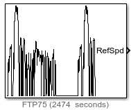
The Drive Cycle Source block generates a standard or user-specified longitudinal drive cycle. The block output is the vehicle longitudinal reference speed as a function of time, along with gear shift schedule if applicable. You can use the drive cycle to:
Predict the required engine torque and fuel consumption for a vehicle to follow a specified speed profile, with a given gear shift schedule.
Produce realistic velocity and shift schedules for closed loop acceleration and braking commands for vehicle control and plant models.
Study, tune, and optimize vehicle control, system performance, and system robustness in covering multiple drive cycles.
Identify faults outside the tolerances specified by standardized tests. These include:
EPA dynamometer driving schedules1
Worldwide Harmonised Light Vehicle Test Procedure (WLTP) laboratory tests2
To generate drive cycles, you can use:
Drive cycles from predefined sources. The block includes the
FTP–75drive cycle by default, and additional cycles can be loaded from a support package.To install additional drive cycles from an add-on, see Install Drive Cycle Data. Certain drive cycles include the gear shift schedules, for example
JC08andCUEDC.Workspace variables that define your own drive cycles.
.
mat, .xls, .xlsx, or .txtfiles. This allows you to load other standard drive cycles, or ones you have built.Wide open throttle (WOT) parameters. An initial and a nominal reference speed are set to produce a sudden large change in reference speed, inducing a WOT condition in the vehicle.
To achieve the goals listed in this table, use the specified Drive Cycle Source block parameter options.
| Goal | Action |
|---|---|
Repeat the drive cycle if the simulation run time exceeds the drive cycle length. | Select Repeat cyclically. |
Output the acceleration, as calculated by Savitzky-Golay differentiation. | Select Output acceleration. |
Specify a sample period for discrete applications. | Specify an Output sample period (0 for continuous), dt parameter. |
Update the simulation run time so that it equals the length of the drive cycle. | Click Update simulation time. If a model configuration reference exists, the block does not enable this option. |
Plot the drive cycle in a MATLAB® figure. | Click Plot drive cycle. |
Specify the drive cycle using a workspace variable. | Click Specify variable. The block:
Specify the workspace variable so that it contains time, velocity, and, optionally, the gear shift schedule. |
Specify the drive cycle by selecting a file. This allows you to load standard cycles other than those listed. | Click Select file. The block:
Specify a file that contains time, velocity, and, optionally, the gear shift schedule. |
Output the drive cycle gear. |
First specify a drive cycle that contains a gear shift schedule. You can use:
Then click Output gear shift data. |
Install additional drive cycles from a support package. | Click Install additional drive cycles. The block enables this option if you can install additional drive cycles from a support package. |
Identify drive cycle faults outside the tolerances specified by standardized tests. | On the Fault Tracking tab, use the parameters to specify the fault tolerances. If the vehicle speed is not within the allowable speed range, the block sets a fault condition. |
Fault and Failure Tracking
On the Fault Tracking tab, use the parameters to specify the fault tolerances. If the vehicle speed is not within the allowable range a given reference time, the block sets a fault condition. Examples for EPA and WLTP cycles are shown here:
| Parameter | Description | Setting | |
|---|---|---|---|
EPA Standard1 | WLTP Tests2 | ||
Speed tolerance | Speed tolerance above the highest point and below the lowest point of the drive cycle speed trace within the time tolerance. | 2.0 mph | 2.0 km/h |
Time tolerance | Time that the block uses to determine the allowable speed range. | 1.0 s | 1.0 s |
| Maximum number of faults | Maximum number of faults allowed during the drive cycle without causing fault failure. | Not specified | 10 |
| Maximum single fault time | Maximum fault duration allowed without causing fault failure. | 2.0 s | 1.0 s |
| Maximum total fault time | Maximum allowed accumulated time under fault condition without causing fault failure. | Not specified | Not specified |
The block uses the time tolerance to determine the allowable speed range at the reference time. Within the time span defined by the reference time +/- the time tolerance, the vehicle speed must be within the reference speed range +/- the velocity tolerance, or the block will set a fault condition. These figures illustrate how the block uses the velocity and time tolerances to determine the allowable speed range.
|
|
|
Create Drive Cycles Using Workspace Variables
If you set Drive cycle source to Workspace
variable, you can specify a workspace variable that defines the
drive cycle.
This table provides examples for using workspace variables to create your own drive cycles.
| Workspace Variable | Source Velocity Units | Output Velocity Units | Drive Cycle Plot |
|---|---|---|---|
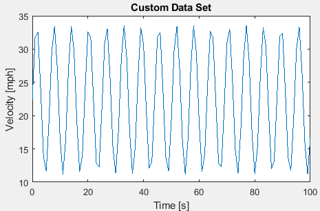
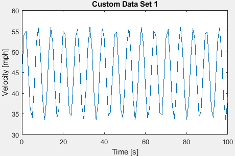
Structure without a gear shift schedule, with From
workspace set to
t = 0:1:100; xdot = 5.*sin(t)+10; myCycleS.time = t'; myCycleS.signals.values = xdot'; | m/s | mph |
|
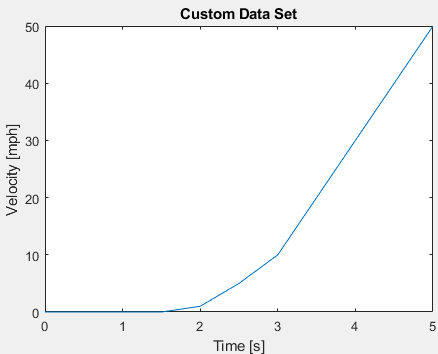
Structure with a gear shift schedule, with From
workspace set to
gears=[0, 1, 2, 3, 3, 4, 4, 4, 4, 4, 4]; t=0:1:10; xdot=[0,5,10,15,20,25,30,30,30,30,30]; myCycleS.time=t'; myCycleS.signals.values=[xdot',gears']; | m/s | mph |
|
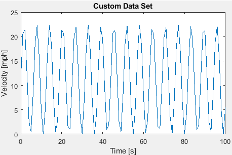
2-D array without a gear shift schedule, with From
workspace set to
t = 0:1:100; xdot = 5.*sin(t)+5; myCycleA = [t',xdot']; | m/s | mph |
|
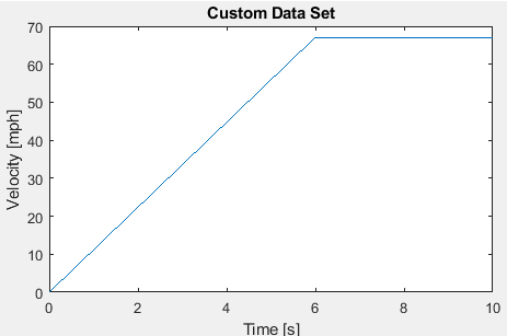
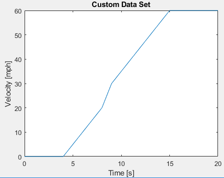
2-D array with a gear shift schedule, with From
workspace set to
gears=[0, 1, 2, 3, 4, 4, 4, 5, 5, 5, 5]; t=0:1:10; xdot=[0,5,10,15,20,25,30,40,50,60,60]; myCycleA=[t',xdot',gears']; | mph | mph |
|
Time series object without a gear shift schedule, with From workspace set
to
myCycleT = timeseries; t = 0:1:100; xdot = 5.*sin(t)+20; myCycleT.Data = xdot'; myCycleT.Time = t'; | m/s | mph |
|
Time series object without a gear shift schedule, with
From workspace set to
myCycleT = timeseries; gears=[0, 1, 2, 3, 4, 4, 4, 5, 5, 5, 5]; t=0:1:10; xdot=[0,10,20,30,32,33,34,40,50,60,60]; myCycleT.Data = [xdot',gears']; myCycleT.Time = t'; | mph | mph |
|


Ports
Input
Output
Parameters
Cycle Setup
Setup
FTP75— Load the FTP75 drive cycle from a .matfile into a 1-D Lookup Table block. The FTP75 represents a city drive cycle that you can use to determine tailpipe emissions and fuel economy of passenger cars.To install additional drive cycles from a support package, see Install Drive Cycle Data.
Wide Open Throttle (WOT)— Use WOT parameters to specify a drive cycle for performance testing.Workspace variable— Specify time, speed, and, optionally, gear data as a structure, 2-D array, or time series object..mat, .xls, .xlsx or .txt file— Specify a file that contains time, speed and, optionally, gear data in column format.
Once you have installed additional cycles, you can use
set_param to set the drive cycle. For example,
to use drive cycle
US06:
set_param([gcs '/Drive Cycle Source'],'cycleVar','US06')
Dependencies
This table summarizes the parameter dependencies.
| Drive Cycle Source | Enables Parameter |
|---|---|
Wide Open Throttle
(WOT) | Start time, t_wot1 |
Initial reference speed, xdot_woto | |
Nominal reference speed, xdot_wot1 | |
Time to start deceleration, t_wot2 | |
Final reference speed, xdot_wot2 | |
WOT simulation time, t_wotend | |
Source velocity units | |
Workspace
variable | From workspace |
Source velocity units | |
Output gear shift data, if drive cycle includes gear shift schedule | |
| Drive cycle source file |
| Source velocity units | |
Output gear shift data, if drive cycle includes gear shift schedule |
Programmatic Use
To set the block
parameter value programmatically, use the set_param
function.
To get the block
parameter value programmatically, use the get_param
function.
| Parameter: | cycleVar |
| Values: | FTP75 (default) | Wide Open Throttle
(WOT) | Workspace variable | .mat, .xls, .xlsx or .txt
file |
| Data Types: | character vector |
A workspace variable containing a monotonically increasing time vector, a velocity vector, and, optionally, a gear data vector. You can use a structure, 2-D array, or time series object. Enter units for velocity in the Source velocity units parameter field.
A valid point must exist for each corresponding time value. You cannot
specify inf, empty, or
NaN.
This table provides examples for using workspace variables to create your own drive cycles.
| Workspace Variable | Source Velocity Units | Output Velocity Units | Drive Cycle Plot |
|---|---|---|---|
Structure without a gear shift schedule, with From
workspace set to
t = 0:1:100; xdot = 5.*sin(t)+10; myCycleS.time = t'; myCycleS.signals.values = xdot'; | m/s | mph |
|
Structure with a gear shift schedule, with From
workspace set to
gears=[0, 1, 2, 3, 3, 4, 4, 4, 4, 4, 4]; t=0:1:10; xdot=[0,5,10,15,20,25,30,30,30,30,30]; myCycleS.time=t'; myCycleS.signals.values=[xdot',gears']; | m/s | mph |
|
2-D array without a gear shift schedule, with From
workspace set to
t = 0:1:100; xdot = 5.*sin(t)+5; myCycleA = [t',xdot']; | m/s | mph |
|
2-D array with a gear shift schedule, with From
workspace set to
gears=[0, 1, 2, 3, 4, 4, 4, 5, 5, 5, 5]; t=0:1:10; xdot=[0,5,10,15,20,25,30,40,50,60,60]; myCycleA=[t',xdot',gears']; | mph | mph |
|
Time series object without a gear shift schedule, with From workspace set
to
myCycleT = timeseries; t = 0:1:100; xdot = 5.*sin(t)+20; myCycleT.Data = xdot'; myCycleT.Time = t'; | m/s | mph |
|
Time series object without a gear shift schedule, with
From workspace set to
myCycleT = timeseries; gears=[0, 1, 2, 3, 4, 4, 4, 5, 5, 5, 5]; t=0:1:10; xdot=[0,10,20,30,32,33,34,40,50,60,60]; myCycleT.Data = [xdot',gears']; myCycleT.Time = t'; | mph | mph |
|
Programmatic Use
To set the block
parameter value programmatically, use the set_param
function.
To get the block
parameter value programmatically, use the get_param
function.
| Parameter: | wsVar |
| Values: | FTP75 (default) | Wide Open Throttle
(WOT) | Workspace variable | .mat, .xls, .xlsx or .txt
file |
| Data Types: | character vector |
Dependencies
To enable this parameter, select Workspace
variable from Drive cycle
source.
File containing monotonically increasing time data, velocity data, and, optionally, gear data in column or comma-separated format. The block ignores units in the file. Enter units for source velocity in the Source velocity units parameter field.
| File | Source Velocity Unit | Output Velocity Unit | Drive Cycle Plot |
|---|---|---|---|
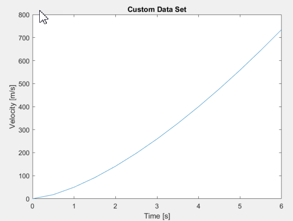
A
. The matrix contains time in column 1 and velocity in column 2. It can optionally contain gear selection in a column 3. sampcyc =
0 0
0.5000 0.7000
1.0000 2.0000
1.5000 3.6000
2.0000 5.6000
2.5000 7.9000
3.0000 10.3000
3.5000 13.0000
4.0000 16.0000
4.5000 19.0000
5.0000 22.3000
5.5000 25.7000
6.0000 29.3000
| m/s | m/s |
|
An
.
| mph | mph |
|
An
.
| mph | mph |
|
A
.
| mph | mph |
|


You can import standard drive cycle file from an external source. For example, you can import the Worldwide Harmonized Motorcycle Emissions Certification and Test Procedure (WMTC) cycle by following the instructions on WTMC. Specifically:
Download the gearshift sheets and instructions.
Follow the instructions to calculate the gear shift data based on your inputs.
The velocity units are
km/hr. Convert the velocity tom/susing the conversion factor 1000/3600.Copy and save the data into a new .
xlsor .xlsxfile for use as a source file.
If you provide the gear schedule using P, R, N, D, L, OD, the block maps the gears to integers.
|
Gear |
Integer |
|---|---|
|
P |
|
|
R |
|
|
N |
|
|
L |
|
|
D |
|
|
OD |
Next integer after highest specified gear. |
For example, the block converts the gear schedule P P N L D 3 4 5 6 5 4
5 6 7 OD 7 to 80 80 0 1 2 3 4 5 6 5 4 5 6 7 8 7.
Programmatic Use
To set the block
parameter value programmatically, use the set_param
function.
To get the block
parameter value programmatically, use the get_param
function.
| Parameter: | fileVar |
| Values: | .mat, .xls, .xlsx or .txt |
| Data Types: | character vector |
Dependencies
To enable this parameter, select .mat, .xls, .xlsx or
.txt file from Drive cycle
source.
Repeat the drive cycle if the simulation run time exceeds the length of the drive cycle.
Programmatic Use
To set the block
parameter value programmatically, use the set_param
function.
To get the block
parameter value programmatically, use the get_param
function.
| Parameter: | cycleRepeat |
| Values: | off (default) | on |
| Data Types: | character vector |
To calculate the acceleration, the block implements Savitzky-Golay differentiation using a second-order polynomial with a three-sample point filter.
Dependencies
To create the output acceleration port, select Output acceleration. Selecting Output acceleration enables the Output acceleration units parameter.
Dependencies
First specify a drive cycle that contains a gear shift schedule. You can use:
A support package to install standard drive cycles that include the gear shift schedules, for example
JC08andCUEDC.Workspace variables.
.
mat, .xls, .xlsx, or .txtfiles.
Clicking this parameter creates input port Gear.
Programmatic Use
To set the block
parameter value programmatically, use the set_param
function.
To get the block
parameter value programmatically, use the get_param
function.
| Parameter: | outGearPort |
| Values: | off (default) | on |
| Data Types: | character vector |
WOT Parameters
Drive cycle start time, in s. For example, this plot shows a drive
cycle with a start time of 10 s.

Programmatic Use
To set the block
parameter value programmatically, use the set_param
function.
To get the block
parameter value programmatically, use the get_param
function.
| Parameter: | t_wot1 |
| Values: | 5 (default) | scalar |
| Data Types: | double |
Dependencies
To enable this parameter, select the Drive cycle source parameter
Wide Open Throttle (WOT).
Initial reference speed, in units that you specify with the
Source velocity units parameter. For example,
this plot shows a drive cycle with an initial reference speed of
4 m/s.
Programmatic Use
To set the block
parameter value programmatically, use the set_param
function.
To get the block
parameter value programmatically, use the get_param
function.
| Parameter: | xdot_woto |
| Values: | 0 (default) | scalar |
| Data Types: | double |
Dependencies
To enable this parameter, select the Drive cycle source parameter
Wide Open Throttle (WOT).
Nominal reference speed, in units that you specify with the
Source velocity units parameter. This is the
maximum speed in the cycle. For example, this plot shows a drive cycle
with a nominal reference speed of 28 m/s.
Programmatic Use
To set the block
parameter value programmatically, use the set_param
function.
To get the block
parameter value programmatically, use the get_param
function.
| Parameter: | xdot_wot1 |
| Values: | 30 (default) | scalar |
| Data Types: | double |
Dependencies
To enable this parameter, select the Drive cycle source parameter
Wide Open Throttle (WOT).
Time to start vehicle deceleration, in s. For example, this plot shows
a drive cycle with vehicle deceleration starting at
25 s.
Programmatic Use
To set the block
parameter value programmatically, use the set_param
function.
To get the block
parameter value programmatically, use the get_param
function.
| Parameter: | t_wot2 |
| Values: | 20 (default) | scalar |
| Data Types: | double |
Dependencies
To enable this parameter, select the Drive cycle source parameter
Wide Open Throttle (WOT).
Final reference speed, in units that you specify with the
Source velocity units parameter. For example,
this plot shows a drive cycle with a final reference speed of
2 m/s.
Programmatic Use
To set the block
parameter value programmatically, use the set_param
function.
To get the block
parameter value programmatically, use the get_param
function.
| Parameter: | xdot_wot2 |
| Values: | 0 (default) | scalar |
| Data Types: | double |
Dependencies
To enable this parameter, select the Drive cycle source parameter
Wide Open Throttle (WOT).
Drive cycle WOT simulation time duration, in s. For example, this plot
shows a drive cycle with a total simulation time of
50 s.
Programmatic Use
To set the block
parameter value programmatically, use the set_param
function.
To get the block
parameter value programmatically, use the get_param
function.
| Parameter: | t_wotend |
| Values: | 30 (default) | scalar |
| Data Types: | double |
Dependencies
To enable this parameter, select the Drive cycle source parameter
Wide Open Throttle (WOT).
Units and Sample Period
Input velocity units.
Programmatic Use
To set the block
parameter value programmatically, use the set_param
function.
To get the block
parameter value programmatically, use the get_param
function.
| Parameter: | srcUnit |
| Values: | m/s (default) |
| Data Types: | character vector |
Dependencies
To enable this parameter, select the Drive cycle source parameter
Wide Open Throttle (WOT), Workspace
variable, or .mat, .xls, .xlsx or .txt
file.
Specify the output acceleration units.
Programmatic Use
To set the block
parameter value programmatically, use the set_param
function.
To get the block
parameter value programmatically, use the get_param
function.
| Parameter: | outAccUnit |
| Values: | m/s^2 (default) |
| Data Types: | character vector |
Dependencies
To enable this parameter, select Output acceleration.
Sample period. Set to 0 for continuous sampling.
For discrete sampling, specify a non-zero period.
Programmatic Use
To set the block
parameter value programmatically, use the set_param
function.
To get the block
parameter value programmatically, use the get_param
function.
| Parameter: | dt |
| Values: | 0 (default) | scalar |
| Data Types: | double |
Fault Tracking
Fault Settings
Select this parameter to enable drive cycle fault tracking. Use the parameters to specify the fault tolerances. If the vehicle speed is not within the allowable speed range, the block sets a fault condition.
Programmatic Use
To set the block
parameter value programmatically, use the set_param
function.
To get the block
parameter value programmatically, use the get_param
function.
| Parameter: | faultOption |
| Values: | off (default) | on |
| Data Types: | character vector |
Dependencies
Selecting this parameter enables these parameters:
Speed tolerance, velBnd
Speed tolerance units, velBndUnit
Velocity feedback units, inUnit
Time tolerance, timeBnd
Standardized tests specify the speed tolerance to use. Here are two examples:
EPA dynamometer driving schedules —
2.0WLTP tests —
2.0
Note that the units for the EPA schedule are mph and for the WLTP tests are km/h.
The block uses the speed tolerance to determine the allowable speed range at the reference time. Within the time span defined by the reference time +/- the time tolerance, the vehicle speed must be within the reference speed range +/- the velocity tolerance, or the block will set a fault condition. These figures illustrate how the block uses the velocity and time tolerances to determine the allowable speed range.
|
|
|
Programmatic Use
To set the block
parameter value programmatically, use the set_param
function.
To get the block
parameter value programmatically, use the get_param
function.
| Parameter: | velBnd |
| Values: | 2.0 (default) | scalar |
| Data Types: | double |
Dependencies
To enable this parameter, on the Fault Tracking tab, select Enable fault tracking.
Standardized tests specify the units for speed tolerance. Here are two examples:
EPA dynamometer driving schedules —
mphWLTP tests —
km/h
Programmatic Use
To set the block
parameter value programmatically, use the set_param
function.
To get the block
parameter value programmatically, use the get_param
function.
| Parameter: | velBndUnit |
| Values: | mph (default) |
| Data Types: | character vector |
Dependencies
To enable this parameter, on the Fault Tracking tab, select Enable fault tracking.
Velocity feedback units. Set the value to the
VelFdbk input port signal units.
Programmatic Use
To set the block
parameter value programmatically, use the set_param
function.
To get the block
parameter value programmatically, use the get_param
function.
| Parameter: | inUnit |
| Values: | m/s (default) |
| Data Types: | character vector |
Dependencies
To enable this parameter, on the Fault Tracking tab, select Enable fault tracking.
The time tolerance, in units of seconds. Standardized tests specify the time tolerance to use. Here are two examples:
EPA dynamometer driving schedules —
1.0WLTP tests —
1.0
The block uses the time tolerance to determine the allowable speed range at the reference time. Within the time span defined by the reference time +/- the time tolerance, the vehicle speed must be within the reference speed range +/- the velocity tolerance, or the block will set a fault condition. These figures illustrate how the block uses the velocity and time tolerances to determine the allowable speed range.
|
|
|
Programmatic Use
To set the block
parameter value programmatically, use the set_param
function.
To get the block
parameter value programmatically, use the get_param
function.
| Parameter: | timeBnd |
| Values: | 1.0 (default) | scalar |
| Data Types: | double |
Dependencies
To enable this parameter, on the Fault Tracking tab, select Enable fault tracking.
Failure Settings
Select this parameter to enable drive cycle failure tracking.
Programmatic Use
To set the block
parameter value programmatically, use the set_param
function.
To get the block
parameter value programmatically, use the get_param
function.
| Parameter: | failOption |
| Values: | off (default) | on |
| Data Types: | character vector |
Dependencies
To enable this parameter, select Enable fault tracking. Selecting Enable failure tracking parameter enables these parameters:
Stop simulation when trace fails, stopSim
Maximum number of faults, maxFaultCnt
Maximum single fault time, maxFaultTime
Maximum total fault time, maxTotFaultTime
Select this parameter to stop the simulation when the trace fails.
To enable this parameter, on the Fault Tracking tab, select Enable failure tracking.
Programmatic Use
To set the block
parameter value programmatically, use the set_param
function.
To get the block
parameter value programmatically, use the get_param
function.
| Parameter: | stopSim |
| Values: | off (default) | on |
| Data Types: | character vector |
Maximum number of faults allowed during the drive cycle. For the number specified by the standardized tests, use these settings:
EPA dynamometer driving schedules — Not specified
WLTP tests —
10
If the number of faults exceeds the maximum number of faults, the block sets a fault failure.
Programmatic Use
To set the block
parameter value programmatically, use the set_param
function.
To get the block
parameter value programmatically, use the get_param
function.
| Parameter: | maxFaultCnt |
| Values: | 10 (default) | scalar |
| Data Types: | double |
Dependencies
To enable this parameter, on the Fault Tracking tab, select Enable failure tracking.
Maximum duration of single fault, in s. For the time specified by the standardized tests, use these settings:
EPA dynamometer driving schedules —
2.0WLTP tests —
1.0
If any fault duration exceeds the maximum single fault time, the block sets a fault failure.
Programmatic Use
To set the block
parameter value programmatically, use the set_param
function.
To get the block
parameter value programmatically, use the get_param
function.
| Parameter: | maxFaultTime |
| Values: | 2.0 (default) | scalar |
| Data Types: | double |
Dependencies
To enable this parameter, on the Fault Tracking tab, select Enable failure tracking.
Maximum accumulated time spent under fault condition, in s.
If the accumulated time spent under fault condition exceeds the maximum total fault time, the block sets a fault failure.
Programmatic Use
To set the block
parameter value programmatically, use the set_param
function.
To get the block
parameter value programmatically, use the get_param
function.
| Parameter: | maxTotFaultTime |
| Values: | 15.0 (default) | scalar |
| Data Types: | double |
Dependencies
To enable this parameter, on the Fault Tracking tab, select Enable failure tracking.
Simulation Trace
Select this parameter to display a velocity trace window. Selecting this parameter can slow the simulation time.
Programmatic Use
To set the block
parameter value programmatically, use the set_param
function.
To get the block
parameter value programmatically, use the get_param
function.
| Parameter: | traceOption |
| Values: | off (default) | on |
| Data Types: | character vector |
Dependencies
Selecting this parameter enables these parameters:
Simulation trace update rate, dtTrace
Simulation trace display window, traceWindow
Simulation trace update period, in s. Set to 0 for
continuous sample period. For a discrete period, specify a non-zero
rate.
Programmatic Use
To set the block
parameter value programmatically, use the set_param
function.
To get the block
parameter value programmatically, use the get_param
function.
| Parameter: | dtTrace |
| Values: | 1 (default) | scalar |
| Data Types: | double |
Dependencies
To enable this parameter, on the Fault Tracking tab, select Display simulation trace.
Simulation trace window update rate, in s.
Programmatic Use
To set the block
parameter value programmatically, use the set_param
function.
To get the block
parameter value programmatically, use the get_param
function.
| Parameter: | traceWindow |
| Values: | 10 (default) | scalar |
| Data Types: | double |
Dependencies
To enable this parameter, on the Fault Tracking tab, select Display simulation trace.
Alternative Configurations
References
[1] Environmental Protection Agency (EPA). EPA urban dynamometer driving schedule. 40 CFR 86.115-78, July 1, 2001.
[2] European Union Commission. "Speed trace tolerances". European Union Commission Regulation. 32017R1151, Sec 1.2.6.6, June 1, 2017.