i-vector Score Calibration

An i-vector system outputs a raw score specific to the data and parameters used to develop the system. This makes interpreting the score and finding a consistent decision threshold for verification tasks difficult.

To address these difficulties, researchers developed score normalization and score calibration techniques.

• In score normalization, raw scores are normalized in relation to an 'imposter cohort'. Score normalization occurs before evaluating the detection error tradeoff and can improve the accuracy of a system and its ability to adapt to new data.

• In score calibration, raw scores are mapped to probabilities, which in turn are used to better understand the system's confidence in decisions.

In this example, you apply score calibration to an i-vector system. To learn about score normalization, see i-vector Score Normalization.

For example purposes, you use cosine similarity scoring (CSS) throughout this example. The interpretability of probabilistic linear discriminant analysis (PLDA) scoring is also improved by calibration.

Starting in R2022a, you can use the calibrate method of ivectorSystem to calibrate both CSS and PLDA scoring.

Download i-vector System and Data Set

To download a pretrained i-vector system suitable for speaker recognition, call speakerRecognition. The ivectorSystem returned was trained on the LibriSpeech data set, which consists of English-language 16 kHz recordings.

ivs = speakerRecognition;

Download the PTDB-TUG data set [1]. The supporting function, loadDataset, downloads the data set and then resamples it from 48 kHz to 16 kHz, which is the sample rate that the i-vector system was trained on. The loadDataset function returns these audioDatastore objects:

• adsEnroll - Contains files to enroll speakers into the i-vector system.

• adsDev - Contains a large set of files to analyze the detection error tradeoff of the i-vector system, and to spot-check performance.

• adsCalibrate - Contains a set of speakers used to calibrate the i-vector system. The calibration set does not overlap with the enroll and dev sets.

targetSampleRate = ivs.SampleRate;
[adsEnroll,adsDev,adsCalibrate] = loadDataset(targetSampleRate);

Starting parallel pool (parpool) using the 'local' profile ...
Connected to the parallel pool (number of workers: 6).

Score Calibration

In score calibration, you apply a warping function to scores so that they are more easily and consistently interpretable as measures of confidence. Generally, score calibration has no effect on the performance of a verification system because the mapping is an affine transformation. The two most popular approaches to calibration are Platt scaling and isotonic regression. Isotonic regression usually results in better performance, but is more prone to overfitting if the calibration data is too small [2].

In this example, you perform calibration using both Platt scaling and isotonic regression, and then compare the calibrations using reliability diagrams.

Extract i-vectors

To properly calibrate a system, you must use data that does not overlap with the evaluation data. Extract i-vectors from the calibration set. You will use these i-vectors to create a calibration warping function.

calibrationIvecs = ivector(ivs,adsCalibrate);

Score i-vector Pairs

You will score each i-vector against each other i-vector to create a matrix of scores, some of which correspond to target scores where both i-vectors belong to the same speaker, and some of which correspond to non-target scores where the i-vectors belong to two different speakers. First, create a targets matrix to keep track of which scores are target and which are non-target.

targets = true(size(calibrationIvecs,2),size(calibrationIvecs,2));
calibrationLabels = adsCalibrate.Labels;
for ii = 1:size(calibrationIvecs,2)
    targets(:,ii) = ismember(calibrationLabels,calibrationLabels(ii));
end

Discard the target scores that corresponds to the i-vector scored with itself by setting the corresponding value in the target matrix to NaN. The supporting function, scoreTargets, scores each valid i-vector pair and returns the results in cell arrays of target and non-target scores.

targets = targets + diag(diag(targets)*nan);
[targetScores,nontargetScores] = scoreTargets(calibrationIvecs,calibrationIvecs,targets);

Use the supporting function, plotScoreDistrubtions, to plot the target and non-target score distributions for the group. The scores range from around 0.64 to 1. In a properly calibrated system, scores should range from 0 to 1. The job of calibrating a binary classification system is to map the raw score to a score between 0 and 1. The calibrated score should be interpretable as the probability that the score corresponds to a target pair.

plotScoreDistributions(targetScores,nontargetScores,Analyze="group")

Platt Scaling

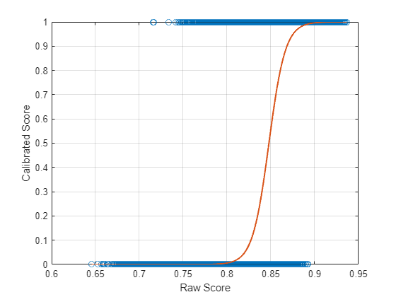
Platt scaling (also referred to as Platt calibration or logistic regression) works by fitting a logistic regression model to a classifier's scores.

The supporting function logistic implements a general logistic function defined as

$$\mathit{p}\left(\mathit{x}\right)=\frac{1}{1+{\mathit{e}}^{\left(\mathit{B}+\mathit{Ax}\right)}}$$

where $\mathit{A}$ and $\mathit{B}$ are the scalar learned parameters.

The supporting function logRegCost defines the cost function for logistic regression as defined in [3]:

$$\stackrel{\mathrm{argmin}}{\mathit{A},\mathit{B}}\left\{-\sum _{\mathit{i}}^{}{\mathit{y}}_{\mathit{i}}\log \left({\mathit{p}}_{\mathit{i}}\right)+\left(1-{\mathit{y}}_{\mathit{i}}\right)\log \left(1-{\mathit{p}}_{\mathit{i}}\right)\right\}$$

As described in [3], the target values are modified from 0 and 1 to avoid overfitting:

$${\mathit{y}}_{+}=\frac{{\mathit{N}}_{+}+1}{{\mathit{N}}_{+}+2};{\mathit{y}}_{-}=\frac{1}{{\mathit{N}}_{-}+2}$$

where ${\mathit{y}}_{+}$ is the positive sample value and ${\mathit{N}}_{+}$ is the number of positive samples, and ${\mathit{y}}_{-}$ is the negative sample value and ${\mathit{N}}_{-}$ is the number of negative samples.

Create a vector of the raw target and non-target scores.

tS = cat(1,targetScores{:});
ntS = cat(1,nontargetScores{:});
x = [tS;ntS];

Create a vector of ideal target probabilities.

yplus = (numel(tS) + 1)./(numel(tS) + 2);
yminus = 1./(numel(ntS) + 2);
y = [yplus*ones(numel(tS),1);yminus*ones(numel(ntS),1)];

Use fminsearch to find the values of A and B that minimize the cost function.

init = [1,1];
AB = fminsearch(@(AB)logRegCost(y,x,AB),init);

Sort the scores in ascending order for visualization purposes.

[x,idx] = sort(x,"ascend");
trueLabel = [ones(numel(tS),1);zeros(numel(ntS),1)];
trueLabel = trueLabel(idx);

Use the supporting function calibrateScores to calibrate the raw scores. Plot the warping function that maps the raw scores to the calibrated scores. Also plot the target scores you are modeling.

calibratedScores = calibrateScores(x,AB);

plot(x,trueLabel,"o")
hold on
plot(x,calibratedScores,LineWidth=1.5)
grid on
xlabel("Raw Score")
ylabel("Calibrated Score")
hold off

Isotonic Regression

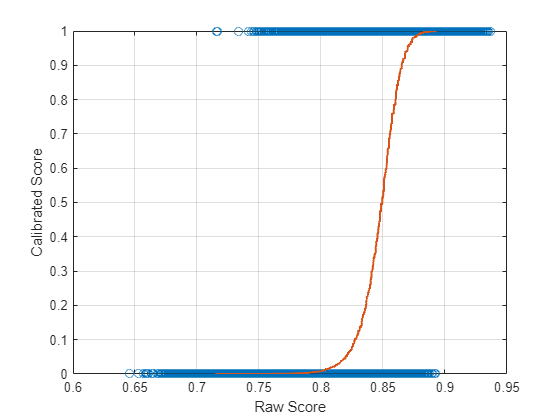
Isotonic regression fits a free-form line to observations with the only condition being that it is non-decreasing (or non-increasing). The supporting function isotonicRegression uses the pool adjacent violators (PAV) algorithm [3] for isotonic regression.

Call isotonicRegression with the raw score and true labels. The function outputs a struct containing a map between raw scores and calibrated scores.

scoringMap = isotonicRegression(x,trueLabel);

Plot the raw score against the calibrated score. The line is the learned isotonic fit. The circles are the data you are fitting.

plot(x,trueLabel,"o")
hold on
plot(scoringMap.Raw,scoringMap.Calibrated,LineWidth=1.5)
grid on
xlabel("Raw Score")
ylabel("Calibrated Score")
hold off

Reliability Diagram

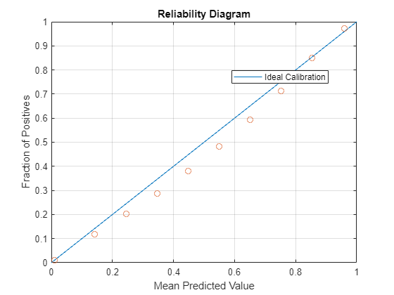
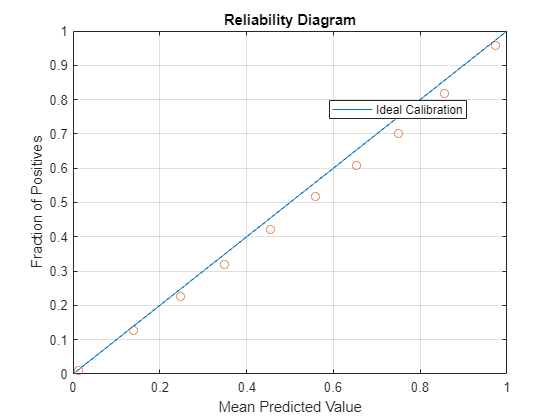
Reliability diagrams reveal reliability by plotting the mean of the predicted value against the known fraction of positives. A system is reliable if the mean of the predicted value is equal to the fraction of positives [4].

Reliability must be assessed using a different data set than the one used to calibrate the system. Extract i-vectors from the development data set, adsDev. The development data set has no speaker overlap with the calibration data set.

devIvecs = ivector(ivs,adsDev);

Create a targets map and score all i-vector pairs.

devLabels = adsDev.Labels;
targets = true(size(devIvecs,2),size(devIvecs,2));
for ii = 1:size(devIvecs,2)
    targets(:,ii) = ismember(devLabels,devLabels(ii));
end
targets = targets + diag(diag(targets)*nan);

[targetScores,nontargetScores] = scoreTargets(devIvecs,devIvecs,targets);

Combine all the scores and labels for faster processing.

ts = cat(1,targetScores{:});
nts = cat(1,nontargetScores{:});
scores = [ts;nts];
trueLabels = [true(numel(ts),1);false(numel(nts),1)];

Calibrate the scores using Platt scaling.

calibratedScoresPlattScaling = calibrateScores(scores,AB);

Calibrate the scores using isotonic regression.

calibratedScoresIsotonicRegression = calibrateScores(scores,scoringMap);

When interpreting the reliability diagram, values below the diagonal indicate that the system is giving higher probability scores than it should be, and values above the diagonal indicate the system is giving lower probability scores than it should. In both cases, increasing the amount of calibration data, and using calibration data like the target application, should improve performance.

numBins = 10;

Plot the reliability diagram for the i-vector system calibrated using Platt scaling.

reliabilityDiagram(trueLabels,calibratedScoresPlattScaling,numBins)

Plot the reliability diagram for the i-vector system calibrated using isotonic regression.

reliabilityDiagram(trueLabels,calibratedScoresIsotonicRegression,numBins)

Supporting Functions

Load Dataset

function [adsEnroll,adsDev,adsCalibrate] = loadDataset(targetSampleRate)
%LOADDATASET Load PTDB-TUG data set
% [adsEnroll,adsDev,adsCalibrate] = loadDataset(targetSampleteRate)
% downloads the PTDB-TUG data set, resamples it to the specified target
% sample rate and save the results in your current folder. The function
% then creates and returns three audioDatastore objects. The enrollment set
% includes two utterances per speaker. The calibrate set does not overlap
% with the other data sets.

% Copyright 2021-2022 The MathWorks, Inc.

rng(0)
downloadFolder = matlab.internal.examples.downloadSupportFile("audio","ptdb-tug.zip");
dataFolder = tempdir;
unzip(downloadFolder,dataFolder)
dataset = fullfile(dataFolder,"ptdb-tug");

% Resample the dataset and save to current folder if it doesn't already
% exist.
if ~isfolder(fullfile(pwd,"MIC"))
    ads = audioDatastore([fullfile(dataset,"SPEECH DATA","FEMALE","MIC"),fullfile(dataset,"SPEECH DATA","MALE","MIC")], ...
        IncludeSubfolders=true, ...
        FileExtensions=".wav", ...
        LabelSource="foldernames");
    reduceDataset = false;
    if reduceDataset
        ads = splitEachLabel(ads,10);
    end
    adsTransform = transform(ads,@(x,y)fileResampler(x,y,targetSampleRate),IncludeInfo=true);
    writeall(adsTransform,pwd,OutputFormat="flac",UseParallel=canUseParallelPool)
end

% Create a datastore that points to the resampled dataset. Use the folder
% names as the labels.
ads = audioDatastore(fullfile(pwd,"MIC"),IncludeSubfolders=true,LabelSource="foldernames");

% Split the data set into enrollment, development, and calibration sets.
calibrationLabels = categorical(["M01","M03","M05","M7","M9","F01","F03","F05","F07","F09"]);

adsCalibrate = subset(ads,ismember(ads.Labels,calibrationLabels));

adsDev = subset(ads,~ismember(ads.Labels,calibrationLabels));

numToEnroll = 2;
[adsEnroll,adsDev] = splitEachLabel(adsDev,numToEnroll);

end

File Resampler

function [audioOut,adsInfo] = fileResampler(audioIn,adsInfo,targetSampleRate)
%FILERESAMPLER Resample audio files
% [audioOut,adsInfo] = fileResampler(audioIn,adsInfo,targetSampleRate)
% resamples the input audio to the target sample rate and updates the info
% passed through the datastore.

% Copyright 2021 The MathWorks, Inc.

arguments
    audioIn (:,1) {mustBeA(audioIn,["single","double"])}
    adsInfo (1,1) {mustBeA(adsInfo,"struct")}
    targetSampleRate (1,1) {mustBeNumeric,mustBePositive}
end

% Isolate the original sample rate
originalSampleRate = adsInfo.SampleRate;

% Resample if necessary
if originalSampleRate ~= targetSampleRate
    audioOut = resample(audioIn,targetSampleRate,originalSampleRate);
    amax = max(abs(audioOut));
    if max(amax>1)
        audioOut = audioOut./amax;
    end
end

% Update the info passed through the datastore
adsInfo.SampleRate = targetSampleRate;

end

Score Targets and Non-Targets

function [targetScores,nontargetScores] = scoreTargets(e,t,targetMap,nvargs)
%SCORETARGETS Score i-vector pairs
% [targetScores,nontargetScores] = scoreTargets(e,t,targetMap) exhaustively
% scores i-vectors in e against i-vectors in t. Specify e as an M-by-N
% matrix, where M corresponds to the i-vector dimension, and N corresponds
% to the number of i-vectors in e. Specify t as an M-by-P matrix, where P
% corresponds to the number of i-vectors in t. Specify targetMap as a
% P-by-N numeric matrix that maps which i-vectors in e and t are target
% pairs (derived from the same speaker) and which i-vectors in e and t are
% non-target pairs (derived from different speakers). Values in targetMap
% set to NaN are discarded. The outputs, targetScores and nontargetScores,
% are N-element cell arrays. Each cell contains a vector of scores between
% the i-vector in e and either all the targets or nontargets in t.
%
% [targetScores,nontargetScores] =
% scoreTargets(e,t,targetMap,NormFactorsSe=NFSe,NormFactorsSt=NFSt)
% normalizes the scores by the specified normalization statistics contained
% in structs NFSe and NFSt. If unspecified, no normalization is applied.

% Copyright 2021 The MathWorks, Inc.

arguments
    e (:,:) {mustBeA(e,["single","double"])}
    t (:,:) {mustBeA(t,["single","double"])}
    targetMap (:,:)
    nvargs.NormFactorsSe = [];
    nvargs.NormFactorsSt = [];
end

% Score the i-vector pairs
scores = cosineSimilarityScore(e,t);

% Apply as-norm1 if normalization factors supplied.
if ~isempty(nvargs.NormFactorsSe) && ~isempty(nvargs.NormFactorsSt)
    scores = 0.5*( (scores - nvargs.NormFactorsSe.mu)./nvargs.NormFactorsSe.std + (scores - nvargs.NormFactorsSt.mu')./nvargs.NormFactorsSt.std' );
end

% Separate the scores into targets and non-targets
targetScores = cell(size(targetMap,2),1);
nontargetScores = cell(size(targetMap,2),1);
removeIndex = isnan(targetMap);
for ii = 1:size(targetMap,2)
    localScores = scores(:,ii);
    localMap = targetMap(:,ii);
    localScores(removeIndex(:,ii)) = [];
    localMap(removeIndex(:,ii)) = [];

    targetScores{ii} = localScores(logical(localMap));
    nontargetScores{ii} = localScores(~localMap);
end
end

Cosine Similarity Score (CSS)

function scores = cosineSimilarityScore(a,b)
%COSINESIMILARITYSCORE Cosine similarity score
% scores = cosineSimilarityScore(a,b) scores matrix of i-vectors, a,
% against matrix of i-vectors b. Specify a as an M-by-N matrix of
% i-vectors. Specify b as an M-by-P matrix of i-vectors. scores is returned
% as a P-by-N matrix, where columns corresponds the i-vectors in a
% and rows corresponds to the i-vectors in b and the elements of the array
% are the cosine similarity scores between them.

% Copyright 2021 The MathWorks, Inc.

arguments
    a (:,:) {mustBeA(a,["single","double"])}
    b (:,:) {mustBeA(b,["single","double"])}
end

scores = squeeze(sum(a.*reshape(b,size(b,1),1,[]),1)./(vecnorm(a).*reshape(vecnorm(b),1,1,[])));
scores = scores';
end

Plot Score Distributions

function plotScoreDistributions(targetScores,nontargetScores,nvargs)
%PLOTSCOREDISTRIBUTIONS Plot target and non-target score distributions
% plotScoreDistribution(targetScores,nontargetScores) plots empirical
% estimations of the distribution for target scores and nontarget scores.
% Specify targetScores and nontargetScores as cell arrays where each
% element contains a vector of speaker-specific scores.
%
% plotScoreDistrubtions(targetScores,nontargetScores,Analyze=ANALYZE)
% specifies the scope for analysis as either "label" or "group". If ANALYZE
% is set to "label", then a score distribution plot is created for each
% label. If ANALYZE is set to "group", then a score distribution plot is
% created for the entire group by combining scores across speakers. If
% unspecified, ANALYZE defaults to "group".

% Copyright 2021 The MathWorks, Inc.

arguments
    targetScores (1,:) cell
    nontargetScores (1,:) cell
    nvargs.Analyze (1,:) char {mustBeMember(nvargs.Analyze,["label","group"])} = "group"
end

% Combine all scores to determine good bins for analyzing both the target
% and non-target scores together.
allScores = cat(1,targetScores{:},nontargetScores{:});
[~,edges] = histcounts(allScores);

% Determine the center of each bin for plotting purposes.
centers = movmedian(edges(:),2,Endpoints="discard");

if strcmpi(nvargs.Analyze,"group")
     % Plot the score distributions for the group.

    targetScoresBinCounts = histcounts(cat(1,targetScores{:}),edges);
    targetScoresBinProb = targetScoresBinCounts(:)./sum(targetScoresBinCounts);
    nontargetScoresBinCounts = histcounts(cat(1,nontargetScores{:}),edges);
    nontargetScoresBinProb = nontargetScoresBinCounts(:)./sum(nontargetScoresBinCounts);

    figure
    plot(centers,[targetScoresBinProb,nontargetScoresBinProb])
    title("Score Distributions")
    xlabel("Score")
    ylabel("Probability")
    legend(["target","non-target"],Location="northwest")
    axis tight

else

    % Create a tiled layout and plot the score distributions for each speaker.

    N = numel(targetScores);
    tiledlayout(N,1)
    for ii = 1:N
        targetScoresBinCounts = histcounts(targetScores{ii},edges);
        targetScoresBinProb = targetScoresBinCounts(:)./sum(targetScoresBinCounts);
        nontargetScoresBinCounts = histcounts(nontargetScores{ii},edges);
        nontargetScoresBinProb = nontargetScoresBinCounts(:)./sum(nontargetScoresBinCounts);
        nexttile
        hold on
        plot(centers,[targetScoresBinProb,nontargetScoresBinProb])
        title("Score Distribution for Speaker " + string(ii))
        xlabel("Score")
        ylabel("Probability")
        legend(["target","non-target"],Location="northwest")
        axis tight
    end
end
end

Calibrate Scores

function y = calibrateScores(score,scoreMapping)
%CALIBRATESCORES Calibrate scores
% y = calibrateScores(score,scoreMapping) maps the raw scores to calibrated
% scores, y, using the score mappinging information in scoreMapping.
% Specify score as a vector or matrix of raw scores. Specify score mapping
% as either struct or a two-element vector. If scoreMapping is specified as
% a struct, then it should have two fields: Raw and Calibrated, that
% together form a score mapping. If scoreMapping is specified as a vector,
% then the elements are used as the coefficients in the logistic function.
% y is returned as vector or matrix the same size as the raw scores.

% Copyright 2021 The MathWorks, Inc.

arguments
    score (:,:) {mustBeA(score,["single","double"])}
    scoreMapping
end

if isstruct(scoreMapping)
    % Calibration using isotonic regression

    rawScore = scoreMapping.Raw;
    interpretedScore = scoreMapping.Calibrated;

    n = numel(score);

    % Find the index of the raw score in the mapping closest to the score provided.
    idx = zeros(n,1);
    for ii = 1:n
        [~,idx(ii)] = min(abs(score(ii)-rawScore));
    end

    % Get the calibrated score.
    y = interpretedScore(idx);

else

    % Calibration using logistic regression
    y = logistic(score,scoreMapping);

end
end

Reliability Diagram

function reliabilityDiagram(targets,predictions,numBins)
%RELIABILITYDIAGRAM Plot reliability diagram
% reliabilityDiagram(targets,predictions) plots a reliability diagram for
% targets and predictions. Specify targets an M-by-1 logical vector.
% Specify predictions as an M-by-1 numeric vector.
%
% reliabilityDiagram(targets,predictions,numBins) specifies the number of
% bins for the reliability diagram. If unspecified, numBins defaults to 10.

% Copyright 2021 The MathWorks, Inc.

arguments
    targets (:,1) {mustBeA(targets,"logical")}
    predictions (:,1) {mustBeA(predictions,["single","double"])}
    numBins (1,1) {mustBePositive,mustBeInteger} = 10;
end

% Bin the predictions into the requested number of bins. Count the number of
% predictions per bin.
[predictionsPerBin,~,predictionsInBin] = histcounts(predictions,numBins);

% Determine the mean of the predictions in the bin.
meanPredictions = accumarray(predictionsInBin,predictions)./predictionsPerBin(:);

% Determine the mean of the targets per bin. This is the fraction of
% positives--the number of targets in the bin over the total number of
% predictions in the bin.
meanTargets = accumarray(predictionsInBin,targets)./predictionsPerBin(:);

plot([0,1],[0,1])
hold on
plot(meanPredictions,meanTargets,"o")
legend("Ideal Calibration",Location="best")
xlabel("Mean Predicted Value")
ylabel("Fraction of Positives")
title("Reliability Diagram")
grid on
hold off

end

Logistic Regression Cost Function

function cost = logRegCost(y,f,iparams)
%LOGREGCOST Logistic regression cost
% cost = logRegCost(y,f,iparams) calculates the cost of the logistic
% function given truth y, prediction f, and logistic params iparams.
% Specify y and f as column vectors. Specify iparams as a two-element row
% vector in the form [A,B], where A and B are the model parameters:
%
%                1
% p(x) = ------------------
%         1 + e^(-A*f - B)
%

% Copyright 2021 The MathWorks, Inc.

arguments
    y (:,1) {mustBeA(y,["single","double"])}
    f (:,1) {mustBeA(f,["single","double"])}
    iparams (1,2) {mustBeA(iparams,["single","double"])}
end
p = logistic(f,iparams);
cost = -sum(y.*log(p) + (1-y).*log(1-p));
end

Logistic Function

function p = logistic(f,iparams)
%LOGISTIC Logistic function
% p = logistic(f,iparams) applies the general logistic function to input f
% with parameters iparams. Specify f as a numeric array. Specify iparams as
% a two-element vector. p is returned as the same size as f.

% Copyright 2021 The MathWorks, Inc.

arguments
    f
    iparams = [1 0];
end
p = 1./(1+exp(-iparams(1).*f - iparams(2)));
end

Isotonic Regression

function scoreMapping = isotonicRegression(x,y)
%ISOTONICREGRESSION Isotonic regression
% scoreMapping = isotonicRegression(x,y) fits a line yhat to data y under
% the monotonicity constraint that x(i)>x(j) -> yhat(i)>=yhat(j). That is,
% the values in yhat are monotontically non-decreasing with respect to x.
% The output, scoreMapping, is a struct containing the changepoints of yhat
% and the corresponding raw score in x.

% Copyright 2021, The MathWorks, Inc.

N = numel(x);

% Sort points in ascending order of x.
[x,idx] = sort(x(:),"ascend"); 
y = y(idx);

% Initialize fitted values to the given values.
m = y;

% Initialize blocks, one per point. These will merge and the number of
% blocks will reduce as the algorithm proceeds.
blockMap = 1:N;
w = ones(size(m));

while true

    diffs = diff(m);
    
    if all(diffs >= 0)

        % If all blocks are monotonic, end the loop.
        break;

    else

        % Find all positive changepoints. These are the beginnings of each
        % block.
        blockStartIndex = diffs>0;

        % Create group indices for each unique block.
        blockIndices = cumsum([1;blockStartIndex]);

        % Calculate the mean of each block and update the weights for the
        % blocks. We're merging all the points in the blocks here.
        m = accumarray(blockIndices,w.*m);
        w = accumarray(blockIndices,w);
        m = m ./ w;

        % Map which block corresponds to which index.
        blockMap = blockIndices(blockMap);

    end
end

% Broadcast merged blocks out to original points.
m = m(blockMap);

% Find the changepoints
changepoints = find(diff(m)>0);
changepoints = [changepoints;changepoints+1];
changepoints = sort(changepoints);

% Remove all points that aren't changepoints.
a = m(changepoints);
b = x(changepoints);

scoreMapping = struct(Raw=b,Calibrated=a);
end

References

[1] G. Pirker, M. Wohlmayr, S. Petrik, and F. Pernkopf, "A Pitch Tracking Corpus with Evaluation on Multipitch Tracking Scenario", Interspeech, pp. 1509-1512, 2011.

[2] van Leeuwen, David A., and Niko Brummer. "An Introduction to Application-Independent Evaluation of Speaker Recognition Systems." Lecture Notes in Computer Science, 2007, 330–53.

[3] Niculescu-Mizil, A., & Caruana, R. (2005). Predicting good probabilities with supervised learning. Proceedings of the 22nd International Conference on Machine Learning - ICML '05. doi:10.1145/1102351.1102430

[4] Brocker, Jochen, and Leonard A. Smith. “Increasing the Reliability of Reliability Diagrams.” Weather and Forecasting 22, no. 3 (2007): 651–61. https://doi.org/10.1175/waf993.1.