Sector Antenna for 2.4GHz Wi-Fi
This example models the inverted Amos sector antenna designed in [1]. A sector antenna is a type of directional antenna with a sector-shaped radiation pattern. The word 'sector' is used here in the geometric sense as a portion of the circumference of a circle measured in degrees.
Inverted Amos Sector Antenna
The antenna consists of a meander dipole (a Franklin antenna) backed by a reflector. The gain of the antenna depends on the number of vertically stacked dipoles in the meander. The current design will use 7 stacked dipoles as shown in Fig.5 in [1]. All other dimensions follow [1].
dipolearms = [88e-3 71e-3 73e-3 65e-3];
wirewidth = cylinder2strip(1e-3);
notchL = 23.8e-3;
notchW = 17e-3;
spacing = 35.5e-3;
GP_length = 660e-3;
GP_Width = 75e-3;
Paper [1] uses the dipole length of 84 mm with a 4 mm feeding gap. Antenna Toolbox™ uses the delta gap feed model. Add the feeding gap length to the length of the dipole resulting in the total length of 88 mm.
Create Antenna
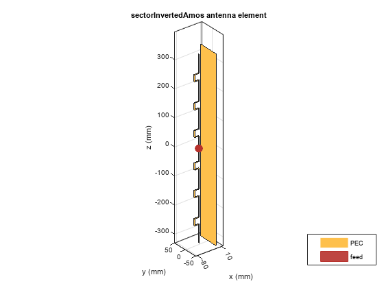
Create the inverted amos sector antenna.
sector = sectorInvertedAmos(ArmWidth=wirewidth, ArmLength=dipolearms,...
     NotchLength=notchL, NotchWidth=notchW, Spacing=spacing,...
     GroundPlaneLength=GP_length, GroundPlaneWidth=GP_Width);
figure
show(sector)
Mesh Structure
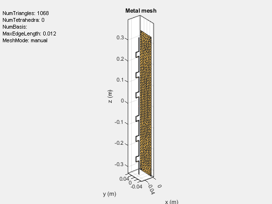
The antenna operates between 2.4 GHz and 2.5 GHz. Manually mesh the structure by using at least 10 elements per wavelength at the highest frequency of the band.
lambda = 3e8/2.5e9;
figure
mesh(sector,MaxEdgeLength=lambda/10);
Radiation Pattern of Sector Antenna
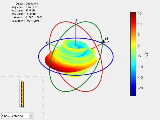
The plots given below show the radiation patterns of the antenna at the center of the Wi-Fi® band at 2.45 GHz. As the antenna name implies, the radiation pattern illuminated a sector with minimum radiation in the back lobe. The maximum directivity is 15.5 dBi, which is slightly higher than the 15.4 dBi reported in [1].
figure
pattern(sector,2.45e9);
view(-45,30)
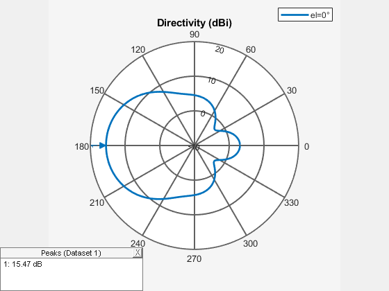
The plots below show the slices of the radiation patterns in the two principle planes.
figure
pattern(sector,2.45e9,0,1:1:360);
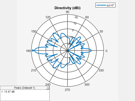
figure
pattern(sector,2.45e9,1:1:360,0);
Antenna Performance Over the Wi-Fi Band
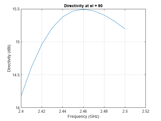
Measure the maximum directivity at an elevation angle of 90 degrees. It is important to have a constant value over the entire band of interest. The plot below, displays the directivity at zenith from 2.4 GHz to 2.5 GHz.
freq = linspace(2.4e9,2.5e9,11);
D = zeros(1,numel(freq));
for m = 1:numel(freq)
    D(m) = pattern(sector, freq(m), 180, 0);
end
figure
plot(freq./1e9, D);
title("Directivity at el = 90");
ylabel("Directivity (dBi)");
xlabel("Frequency (GHz)");
grid on;
Antenna Port Analysis
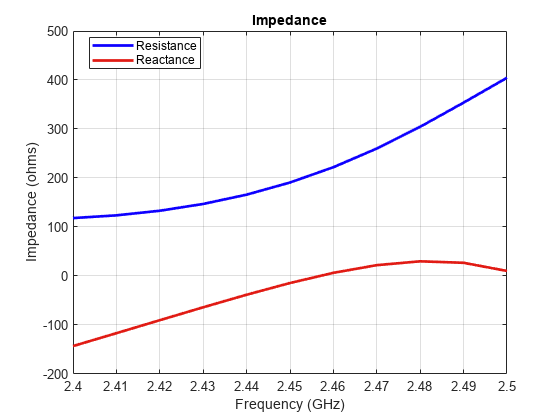
The plot given below shows the input impedance variation of the antenna over the band from 2.4 GHz to 2.5 GHz. The resistance varies between 100 to 400 ohms. To minimize reflections, the antenna is matched to a 200 ohm impedance.
figure
impedance(sector,freq);
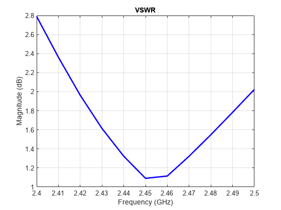
Another way to study the port-based reflection characteristics is to plot the voltage standing wave ratio (VSWR) as well as the reflection coefficient measured with regard to the reference impedance of 200 ohms over the entire Wi-Fi band. The antenna has VSWR around 2 or less and the reflection coefficient around -10 dB or less over the entire frequency band of interest. This indicates an acceptable matching over the Wi-Fi band.
figure
vswr(sector,freq,200);
Calculate the reflection coefficient using the S-parameter data.
S = sparameters(sector,freq,200);
figure
rfplot(S);
title("Reflection coefficient in dB (200 ohms)");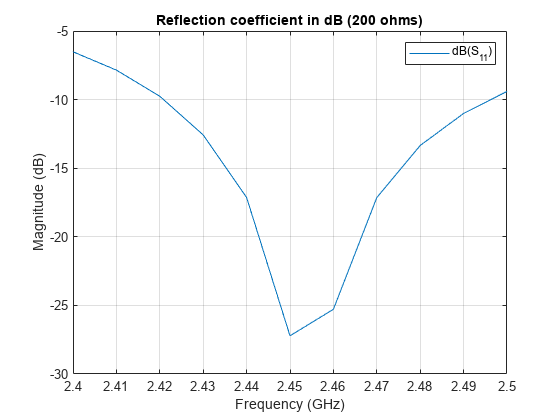
Reference
[1] Inverted Amos Sector Antenna for 2.4 GHz WiFi, AntennaX Issue No. 130, February, 2008.
See Also
Objects
Functions
cylinder2strip|mesh|pattern|impedance|vswr|sparameters