このページの内容は最新ではありません。最新版の英語を参照するには、ここをクリックします。
設計、解析、ベンチマーク、および検証
Antenna Toolbox™ は、一連の解析関数を提供します。これらの関数を使用すると、アンテナまたはアレイのカタログに含まれるさまざまな要素に加え、design 関数を使用して設計したアンテナとアレイを解析できます。アンテナを離散化された三角形にメッシュ化し、解析に用いる方程式を解きます。Antenna Toolbox によるシミュレーション結果を、製造したアンテナ、測定結果、技術情報と比較します。
カテゴリ
- 設計および調整
共振を考慮したアンテナおよびアレイの設計を行い、R、L、C の各成分を使用して調整する
- 解析
ポート、表面、および電界の解析、組み込みパターン、パターン乗算
- メッシング
金属アンテナを三角形に、誘電体を四面体にメッシュ化し、解析に用いる方程式を解く
- ソルバー
MoM、物理光学、ハイブリッド MoM-PO、ワイヤー基底、FMM ソルバー
- ベンチマークおよび検証
シミュレーション結果を測定テスト結果および技術情報と比較する
注目の例

Sensitivity Analysis for Antenna Using Monte-Carlo Simulation
Sensitivity analysis of microstrip patch antenna gain using design space sampling.

Design and Analyze Tapered-Slot SIW Filtenna
Create a substrate-integrated-waveguide-based (SIW-based) antipodal filtenna with a modified feeding network.

Direction of Arrival Determination Using Full-Wave Electromagnetic Analysis
Compute the Direction of Arrival (DoA) of far‑field signals using full‑wave electromagnetic analysis of receive antenna arrays, accounting for array configuration and mutual coupling effects.

Radar Cross Section Benchmarking
Radar cross section benchmarking example.

Parallelization of Antenna and Array Analyses
Speed up antenna and array analysis using Parallel Computing Toolbox™.

Wave Impedance
Uses an elementary dipole and loop antenna to analyze the wave impedance behavior of each radiator in space at a single frequency. The region of space around an antenna has been defined in a variety of ways. The most succinct description is using a 2-or 3-region model. One variation of the 2-region model uses the terms near-field and far-field to identify specific field mechanisms that are dominant. The 3-region model, splits the near-field into a transition zone, wherein a weakly radiative mechanism is at work. Other terms that have been used to describe these zones, include, quasi-static field, reactive field, non-radiative field, Fresnel region, induction zone etc. [1]. Pinning these regions down mathematically presents further challenges as observed with the variety of definitions available across different sources [1]. Understanding the regions around an antenna is critical for both an antenna engineer as well as an electromagnetic compatibility (EMC) engineer. The antenna engineer may want to perform near-field measurements and then compute the far-field pattern. To the EMC engineer, understanding the wave impedance is required for designing a shield with a particular impedance to keep interference out.
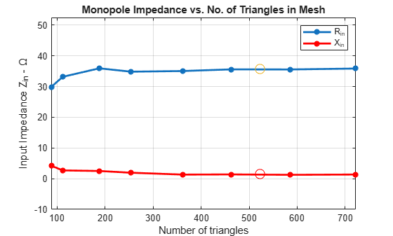
Analysis of Monopole Impedance
Analyzes the impedance behavior of a monopole at varying mesh resolution/sizes and at a single frequency of operation. The resistance and reactance of the monopole are plotted and compared with the theoretical results. A relative convergence curve is established for the impedance.

Analysis of Dipole Impedance
Analyzes the impedance behavior of a center-fed dipole antenna for various mesh resolution/sizes at a single frequency of operation. The resistance and reactance of the dipole are compared with the theoretical results. A relative convergence curve is established for the impedance.

Monopole Measurement Comparison
Compares the impedance of a monopole analyzed in Antenna Toolbox™ with the measured results. The corresponding antenna was fabricated and measured at the Center for Metamaterials and Integrated Plasmonics (CMIP), Duke University. The monopole is designed for an operating frequency of 2.5 GHz.
Comparison of Antenna Array Transmit and Receive Manifold
Calculates and compares the transmit and receive manifolds for a basic half-wavelength dipole antenna array. The array manifold is a fundamental property of antenna arrays, both in transmit and receive configurations. The transmit and receive manifolds are theoretically the same due to the reciprocity theorem. This example validates this equality thus providing an important verification of the calculations performed by the Antenna Toolbox™.

Equiangular Spiral Antenna Design Investigation
Compares results published in [1] for a two-arm equiangular spiral antenna on foamclad backing( 1), with those obtained using the toolbox model of the spiral antenna of the same dimensions. The spiral antennas belong to the class of frequency-independent antennas. In theory, such antennas may possess an infinite bandwidth when made infinitely large. In reality, a finite feeding region has to be established and the outer extent of the spiral antenna has to be truncated.

Helical Antenna Design
Studies a helical antenna designed in [2] with regard to the achieved directivity. Helical antennas were introduced in 1947 [1]. Since then, they have been widely used in certain applications such as mobile and satellite communications. Helical antennas are commonly used in an axial mode of operation which occurs when the circumference of the helix is comparable to the wavelength of operation. In this mode, the helical antenna has the maximum directivity along its axis and radiates a circularly-polarized wave.

Crossed-Dipole (Turnstile) Antenna and Array
The turnstile antenna invented in 1936 by Brown [1] is a valuable tool to create a circularly-polarized pattern (RHCP or LHCP). It is commonly used in mobile communications.

Calculate Radiation Efficiency of Antenna
Calculate the radiation efficiency of an antenna or antenna array from the Antenna Toolbox™. The radiation efficiency of an antenna is defined as the ratio of the power radiated by an antenna to the power fed to the excitation port of the antenna. The power loss due to port impedance mismatch is not considered here.