2 次元低損失圧縮
低損失圧縮の目的は、イメージが与えられたときに、許容できる品質の情報を保存しながら、そのイメージを表すのに必要なビット数を最小限に抑えることです。ウェーブレットを使用すると、この問題を効果的に解決することができます。この詳細な一連の圧縮では、ウェーブレット処理自体に加え、量子化、符号化、復号化を反復的に行います。
この例の目的は、さまざまな圧縮法を使用して、グレースケール イメージまたはトゥルーカラー イメージを分解、圧縮、および解凍する方法を示すことです。これらの機能を説明するために、能面のグレースケール イメージとピーマンのトゥルーカラー イメージを考えます。
グローバルしきい値とハフマン符号化による圧縮
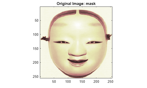
まず、"能面" のグレースケール イメージを読み込んで表示します。
load mask
image(X)
axis square
colormap(pink(255))
title('Original Image: mask')

達成された圧縮の尺度は、圧縮率 (CR) とピクセルあたりのビット数 (BPP) 比によって示されます。CR と BPP は同等の情報を表します。CR は、圧縮されたイメージが初期保存サイズの CR % で保存されることを表します。一方、BPP は、イメージの 1 ピクセルを保存するのに使用されるビット数です。グレースケール イメージの場合、BPP の初期値は 8 です。トゥルーカラー イメージの場合、3 つの色 (RGB 色空間) を符号化するのにそれぞれ 8 ビットが使用されるため、BPP の初期値は 24 です。
圧縮法の課題は、高い圧縮率を得ること (CR の値を小さくすること) と良好な知覚的結果を得ることとの間の最適な妥協点を見つけることです。
まず、グローバル係数のしきい値処理とハフマン符号化をカスケード接続する簡単な方法から始めます。ここでは、既定のウェーブレット "bior4.4" と、指定可能な最大レベル (WMAXLEV 関数を参照) を 2 で割った既定のレベルを使用します。BPP の目標値を 0.5 に設定し、圧縮されたイメージを "mask.wtc" という名前のファイルに保存します。
meth   = 'gbl_mmc_h'; % Method name
option = 'c';         % 'c' stands for compression
[CR,BPP] = wcompress(option,X,'mask.wtc',meth,'BPP',0.5)
CR =
6.7200
BPP =
0.5376
実際に達成されたピクセルあたりのビット数比は約 0.53 (これは目標値の 0.5 に近い) で、圧縮率は 6.7% です。
解凍
ここで、ファイル "mask.wtc" から取得したイメージを解凍し、元のイメージと比較します。
option = 'u';  % 'u' stands for uncompression
Xc = wcompress(option,'mask.wtc');
colormap(pink(255))
subplot(1,2,1); image(X);
axis square;
title('Original Image')
subplot(1,2,2); image(Xc);
axis square;
title('Compressed Image')
xlabel({['Compression Ratio: ' num2str(CR,'%1.2f %%')], ...
        ['BPP: ' num2str(BPP,'%3.2f')]})
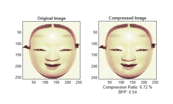
結果は満足のいくものですが、より厳密なしきい値処理と量子化を行う、より洗練された低損失圧縮法を使用することで、圧縮率と画質との間でより良い妥協点を見つけることができます。
段階的な方法による圧縮
ここでは、Haar ウェーブレットを使用した EZW アルゴリズムから始めて段階的に圧縮する方法ついて説明します。重要なパラメーターはループ数です。ループ数を増やすと、再現性は向上しますが、圧縮率は低下します。
meth   = 'ezw';   % Method name
wname  = 'haar';  % Wavelet name
nbloop = 6;       % Number of loops
[CR,BPP] = wcompress('c',X,'mask.wtc',meth,'maxloop', nbloop, ...
                     'wname','haar');
Xc = wcompress('u','mask.wtc');
colormap(pink(255))
subplot(1,2,1); image(X);
axis square;
title('Original Image')
subplot(1,2,2); image(Xc);
axis square;
title('Compressed Image - 6 steps')
xlabel({['Compression Ratio: ' num2str(CR,'%1.2f %%')], ...
        ['BPP: ' num2str(BPP,'%3.2f')]})
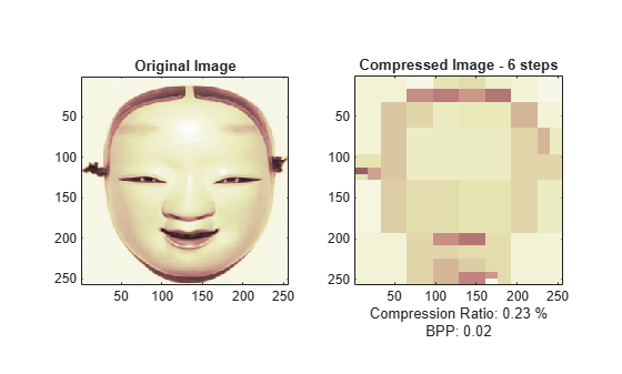
6 ステップのみを使用すると、非常に粗い解凍イメージが生成されます。次に、9 ステップを使用するとわずかに結果が改善され、12 ステップを使用すると満足のいく結果となります。
[CR,BPP] = wcompress('c',X,'mask.wtc',meth,'maxloop',9,'wname','haar');
Xc = wcompress('u','mask.wtc');
colormap(pink(255))
subplot(1,2,1); image(Xc);
axis square;
title('Compressed Image - 9 steps')
xlabel({['Compression Ratio: ' num2str(CR,'%1.2f %%')],...
        ['BPP: ' num2str(BPP,'%3.2f')]})

[CR,BPP] = wcompress('c',X,'mask.wtc',meth,'maxloop',12,'wname','haar');
Xc = wcompress('u','mask.wtc');
subplot(1,2,2); image(Xc);
axis square;
title('Compressed Image - 12 steps')
xlabel({['Compression Ratio: ' num2str(CR,'%1.2f %%')], ...
        ['BPP: ' num2str(BPP,'%3.2f')]})
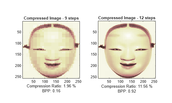
12 ステップを使用した場合、最終的な BPP 比は約 0.92 になります。
ここで、ウェーブレットとして "haar" の代わりに "bior4.4" を使用して結果を改善し、12 ステップと 11 ステップにおけるループ処理の結果を見てみます。
[CR,BPP] = wcompress('c',X,'mask.wtc','ezw','maxloop',12, ...
                     'wname','bior4.4');
Xc = wcompress('u','mask.wtc');
colormap(pink(255))
subplot(1,2,1); image(Xc);
axis square;
title('Compressed Image - 12 steps')
xlabel({['Compression Ratio: ' num2str(CR,'%1.2f %%')], ...
        ['BPP: ' num2str(BPP,'%3.2f')]})

[CR,BPP] = wcompress('c',X,'mask.wtc','ezw','maxloop',11, ...
                     'wname','bior4.4');
Xc = wcompress('u','mask.wtc');
subplot(1,2,2); image(Xc);
axis square;
title('Compressed Image - 11 steps')
xlabel({['Compression Ratio: ' num2str(CR,'%1.2f %%')], ...
        ['BPP: ' num2str(BPP,'%3.2f')]})
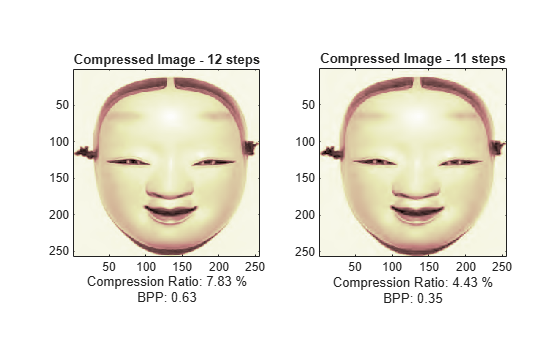
11 回目のループ処理の結果は、満足のいくものと考えられます。このとき、得られた BPP 比は約 0.35 でした。より新しい手法である SPIHT (Set Partitioning in Hierarchical Trees) を使用することで、BPP をさらに改善できます。
[CR,BPP] = wcompress('c',X,'mask.wtc','spiht','maxloop',12, ...
                      'wname','bior4.4');
Xc = wcompress('u','mask.wtc');
colormap(pink(255))
subplot(1,2,1); image(X);
axis square;
title('Original Image')
subplot(1,2,2); image(Xc);
axis square;
title('Compressed Image - 12 steps')
xlabel({['Compression Ratio: ' num2str(CR,'%1.2f %%')], ...
        ['BPP: ' num2str(BPP,'%3.2f')]})
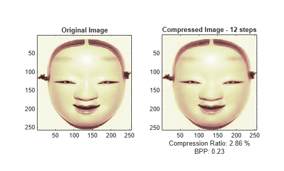
最終的に、圧縮率 2.8%、ピクセルあたりのビット数比 0.23 という非常に満足のいく結果が得られました。この CR は、圧縮されたイメージが初期の保存サイズの 2.8% のみを使用して保存されるという意味であることを思い出してください。
トゥルーカラー イメージの処理
最後に、"wpeppers.jpg" トゥルーカラー イメージを圧縮する方法を説明します。トゥルーカラー イメージは、3 つの色成分のそれぞれに同じ手法を適用することで、グレースケール イメージと同じ方式を使用して圧縮できます。
ここでは、段階的圧縮法として SPIHT (Set Partitioning in Hierarchical Trees) を使用し、符号化処理のループ回数を 12 に設定します。
X = imread('wpeppers.jpg');
[CR,BPP] = wcompress('c',X,'wpeppers.wtc','spiht','maxloop',12);
Xc = wcompress('u','wpeppers.wtc');
colormap(pink(255))
subplot(1,2,1); image(X);
axis square;
title('Original Image')
subplot(1,2,2); image(Xc);
axis square;
title('Compressed Image - 12 steps')
xlabel({['Compression Ratio: ' num2str(CR,'%1.2f %%')], ...
        ['BPP: ' num2str(BPP,'%3.2f')]})

delete('wpeppers.wtc')良好な視認性を維持しながら、圧縮率 1.65%、ピクセルあたりのビット数比 0.4 という非常に満足のいく結果が得られました。
イメージの低損失圧縮の詳細
イメージの低損失圧縮に関する詳しい情報 (理論や例など) については、次の参考文献を参照してください。
Misiti, M., Y. Misiti, G. Oppenheim, J.-M. Poggi (2007), "Wavelets and their applications", ISTE DSP Series.