リフティング
この例では、1 次元信号にリフティングを使用する方法を示します。
2 サンプルにわたって区分的に一定の 1 次元信号を作成します。 のノイズを信号に追加します。
x = [1 1 2 2 -3.5 -3.5 4.3 4.3 6 6 -4.5 -4.5 2.2 2.2 -1.5 -1.5];
x = repmat(x,1,64);
rng default
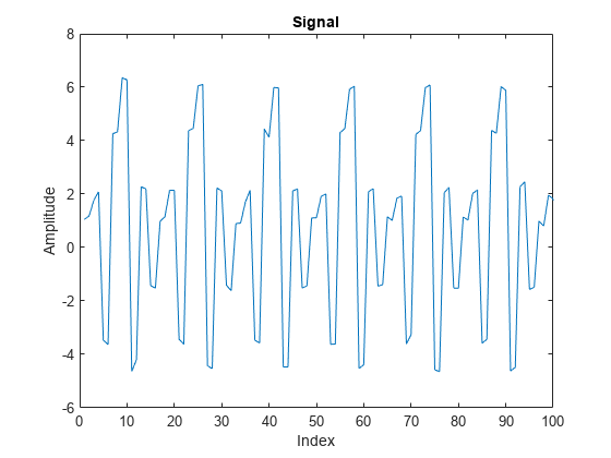
x = x+ 0.1*randn(size(x));信号をプロットし、最初の 100 サンプルを拡大表示して、隣接するサンプルとの相関を可視化します。
plot(x)
xlim([0 100])
title('Signal')
xlabel('Index')
ylabel('Amplitude')
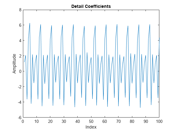
"レイジー" ウェーブレットを使用して、信号の偶数と奇数のポリフェーズ成分を求めます。D の Detail (ウェーブレット) 係数をプロットして、この変換では信号が無相関化されていないことを観測します。ウェーブレット係数は、信号とよく似ているように見えます。
LS = liftingScheme;
[A,D] = lwt(x,'LiftingScheme',LS,'Level',1);
plot(D{1})
xlim([0 100])
title('Detail Coefficients')
xlabel('Index')
ylabel('Amplitude')
偶数のインデックスが付いた係数をその 1 サンプル後の奇数のインデックスが付いた係数から減算する、予測リフティング ステップ を追加します。
ElemLiftStep = liftingStep('Type','predict','Coefficients',-1,'MaxOrder',0);
LSnew = addlift(LS,ElemLiftStep);
信号は連続するサンプル間で区分的に一定で、加法性ノイズを含むため、新しい予測ステップで得られるのは、絶対値が小さいウェーブレット係数です。この場合、ウェーブレット変換はデータを確実に無相関化します。新しい予測ステップで Approximation 係数と Detail 係数を検出して、このことを確認してください。
[A,D] = lwt(x,'liftingScheme',LSnew,'Level',1);
Detail (ウェーブレット) 係数をプロットすると、ウェーブレット係数はもう元の信号とは似ていないことがわかります。
plot(D{1})
xlim([0 100])
title('Detail Coefficients')
xlabel('Index')
ylabel('Amplitude')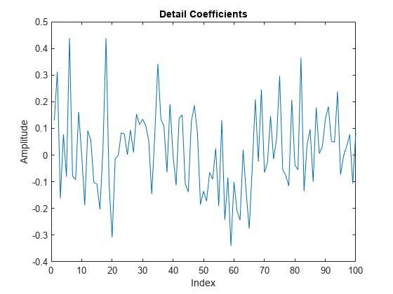
前の変換の Approximation 係数 A は、信号の偶数のポリフェーズ成分を構成します。そのため、これらの係数はエイリアシングの影響を受けます。更新リフティング ステップを使用して Approximation 係数を更新し、エイリアシングを削減します。更新ステップは、Approximation 係数を で置き換えます。これは、 と の平均値です。この平均化は、エイリアシングの削減に役立つローパス フィルター処理です。
ElemLiftStep = liftingStep('Type','update','Coefficients',1/2,'MaxOrder',0);
LSnew = addlift(LSnew,ElemLiftStep);
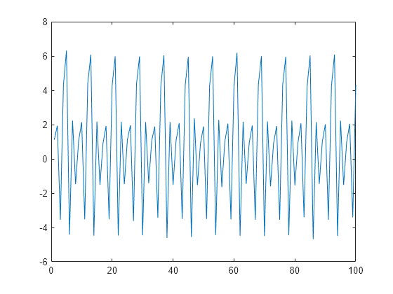
新しい方のリフティング スキームを使用して、入力信号のウェーブレット変換を求めます。Approximation 係数は、元の信号を平滑化したものと似ています。
[A,D] = lwt(x,'liftingScheme',LSnew,'Level',1);
plot(A)
xlim([0 100])
LSnew と同じリフティング ステップで新しいリフティング スキームを作成します。確実に完全再構成が行われるよう、スケーリング係数を適用します。このリフティング スキームを使用して Approximation 係数とウェーブレット係数を求め、ilwt を使用して信号を再構成します。完全再構成されていることを検証します。
scaleFactors = [sqrt(2) sqrt(2)/2];
ElemLiftStep1 = liftingStep('Type','predict','Coefficients',-1,'MaxOrder',0);
ElemLiftStep2 = liftingStep('Type','update','Coefficients',1/2,'MaxOrder',0);
LSscale = liftingScheme('LiftingSteps',[ElemLiftStep1;ElemLiftStep2], ...
    'NormalizationFactors',scaleFactors);
[A,D] = lwt(x,'liftingScheme',LSscale,'Level',1);
xrecon = ilwt(A,D,'liftingScheme',LSscale);
max(abs(x(:)-xrecon(:)))
ans =
1.7764e-15
前の例では、ゼロ次多項式 (定数) を効果的に取り除くウェーブレットを設計しました。高次多項式の方が信号の動作をよく表現できる場合、適切な数の消失モーメントを持つデュアル ウェーブレットを設計して、信号を無相関化できます。
リフティング スキームを使用して、2 つの消失モーメントを持つウェーブレットを設計します。2 つの消失モーメントを持つデュアル ウェーブレットは、1 次多項式で近似される局所的動作を持つ信号を無相関化します。加法性の ノイズを持つ、1 次多項式作用によって特性付けられる信号を作成します。
y = [1 0 0 4 0 0 -1 0 0 2 0 0 7 0 0 -4 0 0 1 0 0 -3];
x1 = 1:(21/1024):22-(21/1024);
y1 = interp1(1:22,y,x1,'linear');
rng default
y1 = y1+0.25*randn(size(y1));
plot(x1,y1)
xlim([1 22])
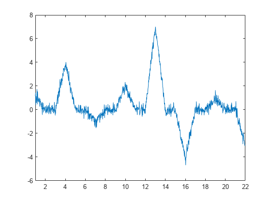
この場合、ウェーブレット係数で 1 次多項式を取り除く必要があります。周辺のサンプル値に当てはめた 1 次多項式によって奇数インデックスの信号の値 が十分に近似される場合、 は を十分に近似するはずです。つまり、 は と の中点になるはずです。
この結果、 は信号を無相関化します。
前の方程式をモデル化する予測リフティング ステップを使用して、新しいリフティング スキームを作成します。
ElemLiftStep = liftingStep('Type','predict','Coefficients',[-1/2 -1/2],'MaxOrder',1);
LS = liftingScheme('LiftingSteps',ElemLiftStep,'NormalizationFactors',1);
リフティング スキームを使用して Approximation 係数と Detail 係数を求め、結果をプロットします。
[A,D] = lwt(y1,'LiftingScheme',LS,'Level',1);
subplot(2,1,1)
plot(A)
xlim([1 512])
title('Approximation Coefficients')
subplot(2,1,2)
plot(D{1})
xlim([1 512])
title('Detail Coefficients')
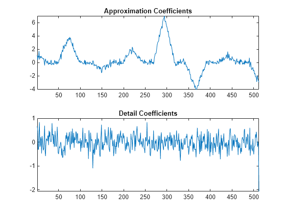
ウェーブレット係数のみがノイズを含んでおり、Approximation 係数が元の信号のノイズ除去されたバージョンを示していることがわかります。前の変換では、Approximation 係数の偶数のポリフェーズ成分のみを使用するため、更新ステップを追加することでエイリアシングを削減できます。
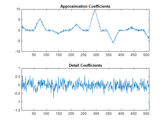
前の予測ステップと、エイリアシングを削減する新しい更新ステップで構成される新しいリフティング スキームを作成します。リフティング スキームを正規化して、完全再構成フィルター バンクを生成します。新しいリフティング スキームで離散ウェーブレット変換を求め、結果をプロットします。
scaleFactors = [sqrt(2) sqrt(2)/2];
ElemLiftStep1 = liftingStep('Type','predict','Coefficients',[-1/2 -1/2],'MaxOrder',1);
ElemLiftStep2 = liftingStep('Type','update','Coefficients',[1/4 1/4],'MaxOrder',0);
LSnew = liftingScheme('LiftingSteps',[ElemLiftStep1;ElemLiftStep2], ...
    'NormalizationFactors',scaleFactors);
[A,D] = lwt(y1,'liftingScheme',LSnew,'Level',1);
subplot(2,1,1)
plot(A)
xlim([1 512])
title('Approximation Coefficients')
subplot(2,1,2)
plot(D{1})
xlim([1 512])
title('Detail Coefficients')
完全再構成フィルター バンクを設計できたことを確認します。
y2 = ilwt(A,D,'liftingScheme',LSnew);
max(abs(y2(:)-y1(:)))
ans = 1.7764e-15