このページは機械翻訳を使用して翻訳されました。最新版の英語を参照するには、ここをクリックします。
XCP 特性のキャリブレーション
この例では、XCP プロトコル機能を使用して、XCP サンプル サーバーに接続し、利用可能な特性データを調整する方法を示します。XCP サンプル サーバーは、XCP の例のみを対象に特別に設計されています。
Vehicle Network Toolbox ™ は、Controller Area Network (CAN)、Controller Area Network Flexible Data-Rate (CAN FD)、Transmission Control Protocol (TCP)、および User Datagram Protocol (UDP) を含む複数のトランスポート層を介してサーバーとインターフェイスするための MATLAB ® 関数を提供します。この例では、パラメータをキャリブレーションし、キャリブレーション前後の測定値を比較します。
XCP は、モデル、アルゴリズム、または ECU の内部パラメータと変数にアクセスして変更するために使用される高レベル プロトコルです。詳細については、ASAM 標準を参照してください。
A2Lファイルを開く
XCP サーバーへの接続を確立するには、A2L ファイルが必要です。A2L ファイルには、XCP サーバーが提供するすべての機能と性能、およびサーバーに接続する方法の詳細が記述されています。xcpA2L 関数を使用して、サーバー モデルを記述する A2L ファイルを開きます。
a2lInfo = xcpA2L("SampleECU.a2l")a2lInfo =
A2L with properties:
File Details
FileName: 'SampleECU.a2l'
FilePath: '/tmp/Bdoc25a_2864802_1974203/tp6f7be44e/vnt-ex60761655/SampleECU.a2l'
ServerName: 'SampleServer'
Warnings: [0×0 string]
Parameter Details
Events: {'Event DAQ 100ms'}
EventInfo: [1×1 xcp.a2l.Event]
Measurements: {'Line' 'PWM' 'Sine'}
MeasurementInfo: [3×1 containers.Map]
Characteristics: {'Gain' 'yData'}
CharacteristicInfo: [2×1 containers.Map]
AxisInfo: [1×1 containers.Map]
RecordLayouts: [3×1 containers.Map]
CompuMethods: [1×1 containers.Map]
CompuTabs: [0×1 containers.Map]
CompuVTabs: [0×1 containers.Map]
XCP Protocol Details
ProtocolLayerInfo: [1×1 xcp.a2l.ProtocolLayer]
DAQInfo: [1×1 xcp.a2l.DAQ]
TransportLayerCANInfo: [1×1 xcp.a2l.XCPonCAN]
TransportLayerUDPInfo: [0×0 xcp.a2l.XCPonIP]
TransportLayerTCPInfo: [1×1 xcp.a2l.XCPonIP]
XCPサンプルサーバーを起動する
XCP サンプル サーバーは、実際の XCP サーバーの動作を制御された方法で模倣します。この場合、機能が制限された例にのみ役立ちます。ローカルのサンプル ECU クラスを使用してサンプル サーバー オブジェクトを作成すると、MATLAB ワークスペースにサンプル サーバーが作成されます。XCP サンプル サーバーは、CAN、CAN FD、および TCP をサポートしています。この例では、デモンストレーションに CAN プロトコルを選択します。
sampleServer = SampleECU(a2lInfo,"CAN","MathWorks","Virtual 1",1);
XCPチャネルを作成する
サーバーへのアクティブな XCP 接続を作成するには、xcpChannel 関数を使用します。この関数には、サーバー A2L ファイルへの参照と、サーバーとのメッセージングに使用するトランスポート プロトコルの種類が必要です。XCP チャネルは、サンプル サーバーと同じデバイスと a2l ファイルを使用して、接続できることを確認する必要があります。
xcpCh = xcpChannel(a2lInfo,"CAN","MathWorks","Virtual 1",1)
xcpCh =
  Channel with properties:

              ServerName: 'SampleServer'
             A2LFileName: 'SampleECU.a2l'
          TransportLayer: 'CAN'
    TransportLayerDevice: [1×1 struct]
              SeedKeyDLL: []
             ConnectMode: 'normal'
サーバーに接続する
サーバーとの通信をアクティブにするには、connect 関数を使用します。
connect(xcpCh);
A2L ファイルから利用可能な特性を表示する
XCP の特性は、モデルのメモリ内の調整可能なパラメータを表します。キャリブレーションに使用できる特性は A2L ファイルで定義されており、Characteristics プロパティにあります。パラメーター Gain は乗数であり、yData は 1 次元ルックアップ テーブルの出力データ ポイントを指定することに注意してください。
a2lInfo.Characteristics
ans = 1×2 cell
    {'Gain'}    {'yData'}
a2lInfo.CharacteristicInfo("Gain")ans =
Characteristic with properties:
Name: 'Gain'
LongIdentifier: 'Scalar SBYTE'
CharacteristicType: VALUE
ECUAddress: 8454145
Deposit: [1×1 xcp.a2l.RecordLayout]
MaxDiff: 0
Conversion: [1×1 xcp.a2l.CompuMethod]
LowerLimit: -100
UpperLimit: 100
Dimension: 1
AxisConversion: {1×0 cell}
BitMask: []
ByteOrder: MSB_LAST
Discrete: []
ECUAddressExtension: 0
Format: '%6.1'
Number: []
PhysUnit: ''
a2lInfo.CharacteristicInfo("yData")ans =
Characteristic with properties:
Name: 'yData'
LongIdentifier: 'Curve with standard axis'
CharacteristicType: CURVE
ECUAddress: 8454912
Deposit: [1×1 xcp.a2l.RecordLayout]
MaxDiff: 0
Conversion: [1×1 xcp.a2l.CompuMethod]
LowerLimit: 0
UpperLimit: 255
Dimension: 8
AxisConversion: {[1×1 xcp.a2l.CompuMethod]}
BitMask: []
ByteOrder: MSB_LAST
Discrete: []
ECUAddressExtension: 0
Format: ''
Number: []
PhysUnit: ''
特性ゲイン値のキャリブレーション
特性 Gain は、値測定 Sine を計算するために使用されます。Gain 値は、測定 Sine の振幅を制御します。
プリロードされた特性値の検査
特性 Gain の現在の値を読み取ります。readCharacteristic 関数は、指定された特性についてサーバーから直接読み取りを実行します。
initialGain = readCharacteristic(xcpCh, "Gain")initialGain = 2
キャリブレーション前に測定値を取得する
測定リストを作成する
この例では、測定値 Sine の値(変更されていない値と 2 つの特性によって変更された値)を調べます。キャリブレーション前後の Sine の連続的に変化する値を可視化するには、DAQ リストを使用して測定データ値を取得します。createMeasurementList 関数を使用して、サーバーからの Sine 測定値を含む DAQ リストを作成します。
createMeasurementList(xcpCh, "DAQ", "Event DAQ 100ms", "Sine", EnableTimestamps = false);
XCP サーバーからデータを取得する
startMeasurement 関数と stopMeasurement 関数を使用して、DAQ リストを短時間実行します。
startMeasurement(xcpCh);
pause(6);
stopMeasurement(xcpCh);
Sine測定データを取得する
Sine 測定の DAQ リストによって取得されたデータを取得するには、readDAQList 関数を使用してから、出力 DAQ リストから Sine 信号を取得します。チャネルには測定リストが 1 つあるため、測定リストのインデックスは 1 になります。
DAQList = readDAQList(xcpCh);
listIndex = 1;
sineBeforeCalibration = DAQList{listIndex}.Sine;
Sine 測定値をプロットする
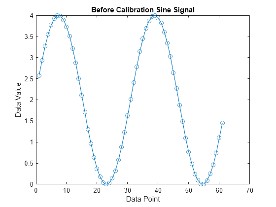
Gain 値を適用した Sine 測定値をプロットします。Sine の測定値は、前述のように、Gain の値が 2 に設定されてブーストされていることを反映しています。
plot(sineBeforeCalibration, "o-");
title("Before Calibration Sine Signal");
xlabel("Data Point");
ylabel("Data Value");
ゲイン特性のキャリブレーション
writeCharacteristic を使用して特性 Gain に新しい値を書き込み、readCharacteristic を使用して読み取りを実行し、変更を確認します。Gain の新しい値は 5 です。つまり、Sine の測定値は新しい Gain 値 5 によってブーストされます。
writeCharacteristic(xcpCh, "Gain", 5);
newGain = readCharacteristic(xcpCh, "Gain")
newGain =
5
キャリブレーション後の測定値の取得
XCP サーバーからデータを取得する
startMeasurement 関数と stopMeasurement 関数を使用して、DAQ リストを短時間実行します。
startMeasurement(xcpCh);
pause(6);
stopMeasurement(xcpCh);
Sine測定データを取得する
Sine 測定の DAQ リストによって取得されたデータを取得するには、readDAQList 関数を使用してから、出力 DAQ リストから Sine 信号を取得します。チャネルには測定リストが 1 つあるため、測定リストのインデックスは 1 になります。
DAQList = readDAQList(xcpCh);
listIndex = 1;
sineAfterCalibration = DAQList{listIndex}.Sine;
Sine 測定値をプロットする
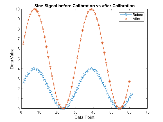
SineAfterCalibration の測定値を SineBeforeCalibration の測定値に対してプロットします。キャリブレーション後に特性 Gain の値が 5 に設定されるため、Sine 測定信号の振幅は高くなります。
plot(sineBeforeCalibration, "o-"); hold on;
plot(sineAfterCalibration, "*-"); hold off;
title("Sine Signal before Calibration vs after Calibration");
legend("Before", "After");
xlabel("Data Point");
ylabel("Data Value");
特性1次元ルックアップテーブルのキャリブレーション
ルックアップ テーブルは、制御パラメータの業界で広く使用されています。したがって、次のセクションでは、XCP サンプル サーバーの軸 xData と特性 yData を使用して 1D ルックアップ テーブルをキャリブレーションする方法を紹介します。
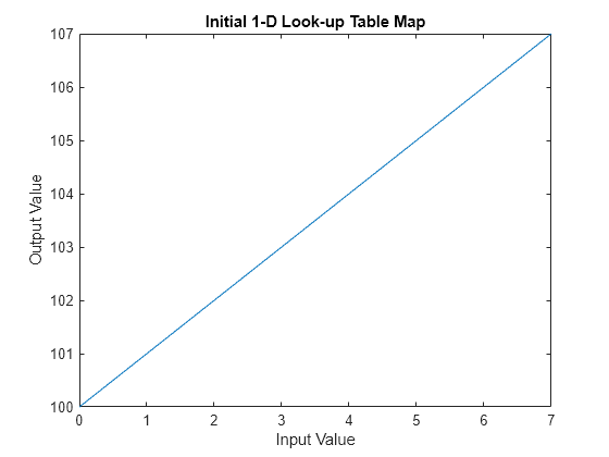
readAxis と readCharacteristic を使用して現在の 1 次元ルックアップ テーブルの特性を読み取り、マッピングをプロットします。このテーブルは、入力値を対応する出力値に効果的にマッピングします。
inputBreakpoints = readAxis(xcpCh, "xData")inputBreakpoints = 1×8
0 1 2 3 4 5 6 7
outputPoints = readCharacteristic(xcpCh, "yData")outputPoints = 1×8
100 101 102 103 104 105 106 107
plot(inputBreakpoints, outputPoints);
title("Initial 1-D Look-up Table Map");
xlabel("Input Value");
ylabel("Output Value");
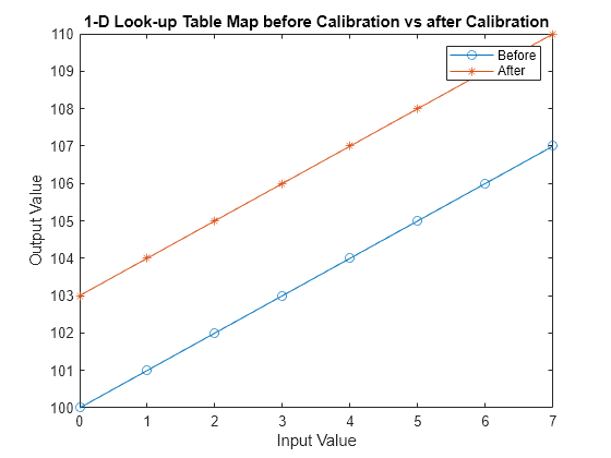
writeCharacteristic を使用して、1 次元ルックアップ テーブルの出力に新しいデータ ポイントを書き込みます。
writeCharacteristic(xcpCh, "yData", 103:110);readAxis と readCharacteristic を使用して新しい 1 次元ルックアップ テーブル データを読み取り、マッピングをプロットします。これで、新しい yData 特性がより高い値に設定されました。
xData = readAxis(xcpCh, "xData");
newOutputPoints = readCharacteristic(xcpCh, "yData")
newOutputPoints = 1×8

   103   104   105   106   107   108   109   110
plot(inputBreakpoints, outputPoints, "o-"); hold on
plot(inputBreakpoints, newOutputPoints, "*-"); hold off;
title("1-D Look-up Table Map before Calibration vs after Calibration");
legend("Before", "After");
xlabel("Input Value");
ylabel("Output Value");
サーバーから切断する
サーバーとの通信を非アクティブにするには、disconnect 関数を使用します。XCP サーバーは、切断後に安全に閉じることができます。
disconnect(xcpCh);
クリーンアップ
clear sampleServer a2lInfo