Symbolic Math Toolbox を使用した Simulink モデルの検証

ライブスクリプトを開く

この例では、古典的な混合力学系である跳ねるボールをモデル化する方法を説明します。このモデルには、連続ダイナミクスと離散遷移の両方が含まれます。ここでは、Symbolic Math Toolbox™ を使用し、跳ねるボールのシミュレーション (Simulink)の常微分方程式を解く背後にある理論のいくつかを説明しています。

仮定

ボールは角度が付かずに跳ね返る
抵抗は存在しない
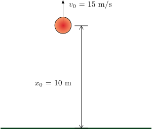
時間 t=0 における高さは 10 m である
上向きの速度 15 m/s で投げる

導出

反発係数は次のように定義されます。

$C_{r} = v_{b} - v_{a} / u_{a} - u_{b}$

ここで、v は衝突前の物体の速度、u は衝突後の速度です。

以下の 2 階微分方程式

$\frac{d^{2} h}{d t^{2}} = - g$

を以下の

$\frac{h (t + Δ t) - h (t)}{Δ t} = v (t)$ として離散化される $\frac{d h}{d t} = v$ に分解します。

さらに

$\frac{v (t + Δ t) - v (t)}{Δ t} = - g$ として離散化される $\frac{d v}{d t} = - g$ に分解します。

前進オイラー法により基本的な 1 階数値積分を使用します。

$h (t + Δ t) = h (t) + v (t) Δ t$

$v (t + Δ t) = v (t) - g Δ t$

問題の解析的な求解

Symbolic Math Toolbox を使用すると、問題に解析的に取り組むことができます。これにより、たとえば、初めてボールが地面に衝突する時点の正確な判定 (以下を参照) などの問題を、より簡単に解くことができます。

シンボリック変数を宣言します。

syms g t H(t) h_0 v_0

2 階微分方程式 $\frac{d^{2} h}{d t^{2}} = - g$ を $\frac{d h}{d t} = v$ と $\frac{d v}{d t} = - g$ に分割します。

Dh = diff(H);
D2h = diff(H, 2) == g

D2h(t) = 
 $\frac{\partial^{2}}{\partial t^{2}} H (t) = g$

dsolve を使用して ODE を解きます。

eqn = dsolve(D2h, H(0) == h_0, Dh(0) == v_0)

eqn = 
 $\frac{g t^{2}}{2} + v_{0} t + h_{0}$

subs を使用して、運動の放物型プロファイルをパラメトリックに調べます。

eqn = subs(eqn, [h_0, v_0, g], [10, 15, -9.81])

eqn = 
 $- \frac{981 t^{2}}{200} + 15 t + 10$

ゼロについて解き、ボールが地面に衝突する時点を求めます。

assume(t > 0)
tHit = solve(eqn == 0)

tHit = 
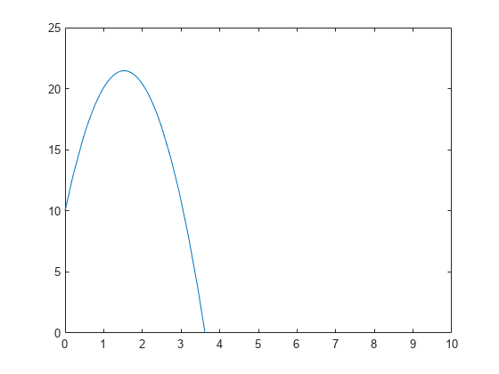
 $\frac{20 \sqrt{5} \sqrt{26}}{109} + \frac{500}{327}$

解を可視化します。

fplot(eqn,[0 10])
ylim([0 25])

vpa で可変精度演算を使用した場合の厳密な結果の書式を設定します。

disp(['The ball with an initial height of 10m and velocity of 15m/s will hit the ground at ' char(vpa(tHit, 4)) ' seconds.'])

The ball with an initial height of 10m and velocity of 15m/s will hit the ground at 3.621 seconds.

問題の数値的な求解

シミュレーションパラメーターの設定

ボールのプロパティ

c_bounce = .9;        % Bouncing's coefficient of restitution; perfect restitution would be 1

シミュレーションのプロパティ

gravity  = 9.8;       % Gravity's acceleration (m/s)
height_0 = 10;        % Initial height at time t=0 (m)
velocity_0=15;        % Initial velocity at time t=0 (m/s)

シミュレーションタイムステップの宣言

dt = 0.05;            % Animation timestep (s)
t_final = 25;         % Simulate period (s)
t = 0:dt:t_final;     % Timespan
N = length(t);        % Number of iterations

シミュレーション量の初期化

h=[];                 % Height of the ball as a function of time (m)
v=[];                 % Velocity of the ball (m/sec) as a function of time (m/s)
h(1)=height_0;
v(1)=velocity_0;

跳ねるボールをシミュレート (前進オイラー法による基本的な 1 階数値積分を使用):

for i=1:N-1
       
    v(i+1)=v(i)-gravity*dt;
    h(i+1)=h(i)+v(i)*dt;
    
    % When the ball bounces (the height is less than 0), 
    % reverse the velocity and recalculate the position.
    % Using the coefficient of restitution
    if h(i+1) < 0
        
       v(i)=-v(i)*c_bounce;
       v(i+1)=v(i)-gravity*dt;
       h(i+1)=0+v(i)*dt;

    end
    
end

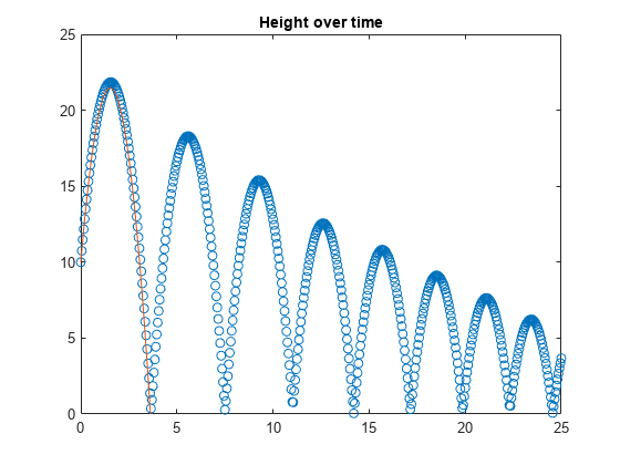
シミュレーションの可視化と検証

plot(t,h,'o')
hold on 
fplot(eqn,[0 10])
title('Height over time')
ylim([0 25])
hold off

plot(t,v)
title('Velocity over time')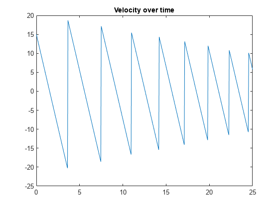

解析値による数値の検証

解析結果と数値結果の比較

衝突の時点は以下でした。

disp(['The ball with an initial height of 10m and velocity of 15m/s will hit the ground at ' char(vpa(tHit, 4)) ' seconds.'])

The ball with an initial height of 10m and velocity of 15m/s will hit the ground at 3.621 seconds.

数値シミュレーションから、 $h (t_{i}) \approx 0$ のときにシミュレーションの値と最も近接することがわかります。

i = ceil(double(tHit/dt));
t([i-1 i i+1])

ans = 1×3

    3.5500    3.6000    3.6500

plot(t,h,'o')
hold on 
fplot(eqn,[0 10])
plot(t([i-1 i i+1 ]),h([i-1 i i+1 ]),'*R')
title('Height over time')
xlim([0 5])
ylim([0 25])
hold off