パデ近似

R2026a

階数が [m, n] のパデ近似は、x = x₀ の周辺で関数 f(x) を次のように近似します。

$\frac{a_{0} + a_{1} (x - x_{0}) + ... + a_{m} {(x - x_{0})}^{m}}{1 + b_{1} (x - x_{0}) + ... + b_{n} {(x - x_{0})}^{n}} .$

パデ近似は 2 つのべき級数の比で構成される有理関数です。これは有理関数なので、極をもつ関数を近似するうえでテイラー級数よりも正確です。パデ近似は Symbolic Math Toolbox™ の関数 pade によって表されます。

展開点 x = x₀ に極または零点が存在すると、パデ近似の精度が低下します。精度を上げるために、次に示すパデ近似の代替形を使用できます。

$\frac{{(x - x_{0})}^{p} (a_{0} + a_{1} (x - x_{0}) + ... + a_{m} {(x - x_{0})}^{m})}{1 + b_{1} (x - x_{0}) + ... + b_{n} {(x - x_{0})}^{n}} .$

入力引数 OrderMode を Relative に設定すると、関数 pade はパデ近似の代替形を返します。

パデ近似は、制御系理論でシステム応答の時間遅延のモデル化に使用されます。時間遅延は、化学処理や輸送プロセスなど、入力とシステム応答の間に遅延があるシステムで発生します。これらの入力をモデル化したものはむだ時間入力と呼ばれます。この例では、Symbolic Math Toolbox でパデ近似を使用して、むだ時間入力に対する 1 次の系の応答をモデル化する方法を説明します。

1 次の系の動作は次の微分方程式によって表されます。

$τ \frac{d y (t)}{d t} + y (t) = a x (t) .$

MATLAB^® にこの微分方程式を入力します。

syms tau a x(t) y(t) xS(s) yS(s) H(s) tmp
F = tau*diff(y)+y == a*x;

laplace を使用して F のラプラス変換を求めます。

F = laplace(F,t,s)

F =  $laplace (y (t), t, s) - τ (y (0) - s laplace (y (t), t, s)) = a laplace (x (t), t, s)$

t = 0 のときのシステムの応答が 0 であると仮定します。subs を y(0) = 0 の代わりに使用します。

F = subs(F,y(0),0)

F =  $laplace (y (t), t, s) + s τ laplace (y (t), t, s) = a laplace (x (t), t, s)$

simplify を使用して共通項をくくります。

F = simplify(F)

F =  $(s τ + 1) laplace (y (t), t, s) = a laplace (x (t), t, s)$

見やすくするため、x(t) と y(t) のラプラス変換を xS(s) と yS(s) で置き換えます。

F = subs(F,[laplace(x(t),t,s) laplace(y(t),t,s)],[xS(s) yS(s)])

F =  $yS (s) (s τ + 1) = a xS (s)$

伝達関数のラプラス変換は yS(s)/xS(s) です。方程式の両辺を xS(s) で除算し、subs を使用して yS(s)/xS(s) を H(s) で置き換えます。

F = F/xS(s);
F = subs(F,yS(s)/xS(s),H(s))

F =  $H (s) (s τ + 1) = a$

H(s) について方程式を解きます。H(s) をダミー変数で置き換え、solve を使用してダミー変数を求め、解を H(s) に代入します。

F = subs(F,H(s),tmp);
H(s) = solve(F,tmp)

H(s) = 
 $\frac{a}{s τ + 1}$

1 次の系への入力は時間遅延を加えたステップ入力です。ステップ入力を表すには heaviside を使用します。入力を 3 時間単位遅らせます。laplace を使用してラプラス変換を求めます。

step = heaviside(t - 3);
step = laplace(step)

step = 
 $\frac{e^{- 3 s}}{s}$

システムの応答、つまり伝達関数と入力の積を求めます。

y = H(s)*step

y = 
 $\frac{a e^{- 3 s}}{s (s τ + 1)}$

応答をプロットするため、パラメーター a と tau に値を設定します。a と tau には、それぞれ1 と 3 を選択します。

y = subs(y,[a tau],[1 3]);
y = ilaplace(y,s);

入力引数 Order を pade に使用して、ステップ入力の階数 [2 2] のパデ近似を求めます。

stepPade22 = pade(step,'Order',[2 2])

stepPade22 = 
 $\frac{3 s^{2} - 4 s + 2}{2 s (s + 1)}$

伝達関数と入力のパデ近似を乗算して入力に対する応答を求めます。

yPade22 = H(s)*stepPade22

yPade22 = 
 $\frac{a (3 s^{2} - 4 s + 2)}{2 s (s τ + 1) (s + 1)}$

ilaplace を使用して yPade22 の逆ラプラス変換を求めます。

yPade22 = ilaplace(yPade22,s)

yPade22 = 
 $a + \frac{9 a e^{- s}}{2 τ - 2} - \frac{a e^{- \frac{s}{τ}} (2 τ^{2} + 4 τ + 3)}{τ (2 τ - 2)}$

応答をプロットするため、パラメーター a と tau の値をそれぞれ 1 と 3 に設定します。

yPade22 = subs(yPade22,[a tau],[1 3])

yPade22 = 
 $\frac{9 e^{- s}}{4} - \frac{11 e^{- \frac{s}{3}}}{4} + 1$

システム y の応答とパテ近似 yPade22 から算出された応答をプロットします。

hold on
grid on
fplot([y yPade22],[0 20])
title('Pade Approximant for dead-time step input')
legend('Response to dead-time step input',...
       'Pade approximant [2 2]',...
       'Location', 'Best')

Figure contains an axes object. The axes object with title Pade Approximant for dead-time step input contains 2 objects of type functionline. These objects represent Response to dead-time step input, Pade approximant [2 2].

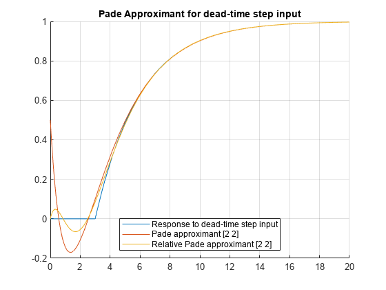
0 の展開点に極が存在するため、[2 2] パデ近似は応答をうまく表していません。展開点に極や零があるときに pade の精度を上げるには、入力引数 OrderMode に Relative を設定し、同じ手順を繰り返します。詳細については、pade を参照してください。

stepPade22Rel = pade(step,'Order',[2 2],'OrderMode','Relative')

stepPade22Rel = 
 $\frac{3 s^{2} - 6 s + 4}{s (3 s^{2} + 6 s + 4)}$

yPade22Rel = H(s)*stepPade22Rel

yPade22Rel = 
 $\frac{a (3 s^{2} - 6 s + 4)}{s (s τ + 1) (3 s^{2} + 6 s + 4)}$

yPade22Rel = ilaplace(yPade22Rel)

yPade22Rel = 
 $\begin{array}{l} a - \frac{a e^{- \frac{t}{τ}} (4 τ^{2} + 6 τ + 3)}{σ_{1}} + \frac{12 a τ e^{- t} (\cos (\frac{\sqrt{3} t}{3}) - \sqrt{3} \sin (\frac{\sqrt{3} t}{3}) (\frac{36 a - 72 a τ}{36 a τ} + 1))}{σ_{1}} \\ where \\ σ_{1} = 4 τ^{2} - 6 τ + 3 \end{array}$

yPade22Rel = subs(yPade22Rel,[a tau],[1 3])

yPade22Rel = 
 $\frac{12 e^{- t} (\cos (\frac{\sqrt{3} t}{3}) + \frac{2 \sqrt{3} \sin (\frac{\sqrt{3} t}{3})}{3})}{7} - \frac{19 e^{- \frac{t}{3}}}{7} + 1$

fplot(yPade22Rel,[0 20],'DisplayName','Relative Pade approximant [2 2]')

Figure contains an axes object. The axes object with title Pade Approximant for dead-time step input contains 3 objects of type functionline. These objects represent Response to dead-time step input, Pade approximant [2 2], Relative Pade approximant [2 2].

また、階数を増やすことでパデ近似の精度を上げることもできます。階数を [4 5] に増やし、同じ手順を繰り返します。t = 0 での応答を近似する点で、[n-1 n] パデ近似は [n n] パデ近似よりも優れています。

stepPade45 = pade(step,'Order',[4 5])

stepPade45 = 
 $\frac{27 s^{4} - 180 s^{3} + 540 s^{2} - 840 s + 560}{s (27 s^{4} + 180 s^{3} + 540 s^{2} + 840 s + 560)}$

yPade45 = H(s)*stepPade45

yPade45 = 
 $\frac{a (27 s^{4} - 180 s^{3} + 540 s^{2} - 840 s + 560)}{s (s τ + 1) (27 s^{4} + 180 s^{3} + 540 s^{2} + 840 s + 560)}$

yPade45 = subs(yPade45,[a tau],[1 3])

yPade45 = 
 $\frac{27 s^{4} - 180 s^{3} + 540 s^{2} - 840 s + 560}{s (3 s + 1) (27 s^{4} + 180 s^{3} + 540 s^{2} + 840 s + 560)}$

yPade45 = ilaplace(yPade45)

yPade45 = 
 $\begin{array}{l} \frac{101520 (\sum_{k = 1}^{4} \frac{e^{σ_{2} t} σ_{2}}{12 (90 σ_{2} + 45 {σ_{2}}^{2} + 9 {σ_{2}}^{3} + 70)})}{143} - \frac{2721 e^{- \frac{t}{3}}}{1001} + \frac{172560 (\sum_{k = 1}^{4} \frac{e^{t σ_{2}}}{σ_{1}})}{143} + \frac{294120 (\sum_{k = 1}^{4} \frac{e^{t σ_{2}} {σ_{2}}^{2}}{σ_{1}})}{1001} + \frac{46440 (\sum_{k = 1}^{4} \frac{e^{t σ_{2}} {σ_{2}}^{3}}{σ_{1}})}{1001} + 1 \\ where \\ σ_{1} = 12 (9 {σ_{2}}^{3} + 45 {σ_{2}}^{2} + 90 σ_{2} + 70) \\ σ_{2} = root (z^{4} + \frac{20 z^{3}}{3} + 20 z^{2} + \frac{280 z}{9} + \frac{560}{27}, z, k) \end{array}$

yPade45 = vpa(yPade45)

yPade45 =  $3.2418384981662546679005910164486 e^{- 1.930807068546914778929595950184 t} \cos (0.57815608595633583454598214328008 t) - 2.7182817182817182817182817182817 e^{- 0.33333333333333333333333333333333 t} - 1.5235567798845363861823092981669 e^{- 1.4025262647864185544037373831494 t} \cos (1.7716120279045018112388813990878 t) + 11.595342871672681856604670597166 e^{- 1.930807068546914778929595950184 t} \sin (0.57815608595633583454598214328008 t) - 1.7803798379230333426855987436911 e^{- 1.4025262647864185544037373831494 t} \sin (1.7716120279045018112388813990878 t) + 1.0$

fplot(yPade45,[0 20],'DisplayName','Pade approximant [4 5]')

Figure contains an axes object. The axes object with title Pade Approximant for dead-time step input contains 4 objects of type functionline. These objects represent Response to dead-time step input, Pade approximant [2 2], Relative Pade approximant [2 2], Pade approximant [4 5].

以下の点を説明しました。

パデ近似はむだ時間ステップ入力をモデル化できる。
パデ近似の精度は、近似の階数の増加に合わせて向上する。
展開点に極または零点が存在すると、展開点周辺ではパデ近似は不正確になる。近似の精度を上げるには、OrderMode オプションを Relative に設定する。分子に対する分母の階数を上げるという方法を使用することもできる。