非負値行列因子分解の実行

この例では、非負値行列因子分解を実行する方法を示します。

標本データを読み込みます。

load moore
X = moore(:,1:5);
rng('default'); % For reproducibility

W と H の 5 つの無作為な初期値から開始する乗法更新アルゴリズムを使用して、X のランク 2 の近似を計算します。

opt = statset('MaxIter',10,'Display','final');
[W0,H0] = nnmf(X,2,'replicates',5,'options',opt,'algorithm','mult');

    rep	   iteration	   rms resid	  |delta x|
      1	      10	     358.296	  0.00190554
      2	      10	     78.3556	 0.000351747
      3	      10	     230.962	   0.0172839
      4	      10	     326.347	  0.00739552
      5	      10	     361.547	  0.00705539
Final root mean square residual = 78.3556

'mult' アルゴリズムは初期値に敏感です。そして、'replicates' を使用して、複数のランダムな開始値から W と H を見つけます。

交互最小二乗アルゴリズムを使用して、因子分解を実行します。このアルゴリズムは、より高速かつ着実に収束します。上記で識別された初期値 W0 と H0 から開始して、反復をさらに 100 回実行します。

opt = statset('Maxiter',1000,'Display','final');
[W,H] = nnmf(X,2,'w0',W0,'h0',H0,'options',opt,'algorithm','als');

    rep	   iteration	   rms resid	  |delta x|
      1	       2	     77.5315	 0.000830334
Final root mean square residual = 77.5315

W の 2 つの列は変換予測子です。H の 2 行は、W 内の予測子に、X 内の 5 つの各予測子の相対的な寄与を与えます。H を表示します。

H

H = 2×5

    0.0835    0.0190    0.1782    0.0072    0.9802
    0.0559    0.0250    0.9969    0.0085    0.0497

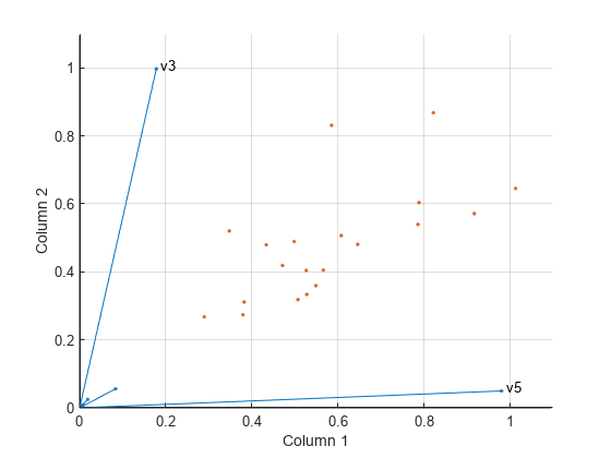
X の 5 番目の予測子 (重みは 0.9802) は、W の 1 番目の予測子に大きい影響を与えます。X の 3 番目の予測子 (重みは 0.9969) は、W の 2 番目の予測子に大きい影響を与えます。

biplot を使用して X の予測子の相対的な寄与を可視化し、W の列空間でデータと元の変数を表示します。

biplot(H','scores',W,'varlabels',{'','','v3','','v5'});
axis([0 1.1 0 1.1])
xlabel('Column 1')
ylabel('Column 2')

参考

nnmf

関連するトピック

• 非負値行列因子分解