Model Hysteresis and Eddy Current Losses in an Iron Core

Since R2024b

This example shows how to model the hysteresis and eddy current losses in the iron core of an electrical transformer using the Magnetic Core block. This block represents a magnetic core with magnetic hysteresis and implements the Jiles-Atherton model. You can parameterize the block using saturated B-H curve data, magnetic characteristics, or the Jiles-Atherton parameters.

Open Model

Open the modelHysteresisEddyTransformerLosses model.

myModel = "modelHysteresisEddyTransformerLosses";
open_system(myModel)

Plot the B-H curve using a fixed frequency and variable amplitude magnetic field intensity input.

modelHysteresisEddyTransformerLossesPlotBHCurve(myModel,Amplitude="Variable",Frequency="Fixed",ModelEddyLosses="false",stopTime=500/f)

 The Jiles-Atherton parameters used for the simulation are: 
 Ms = 994718.3943A/m 
 a = 3652.6652A/m 
 alpha = 0.0094825 
 c = 0.001 
 k = 3978.4325A/m 

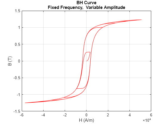
The model simulates the inner and saturated hysteresis cycles. The curve is within the bounds of the saturation values.

Model Hysteresis Losses

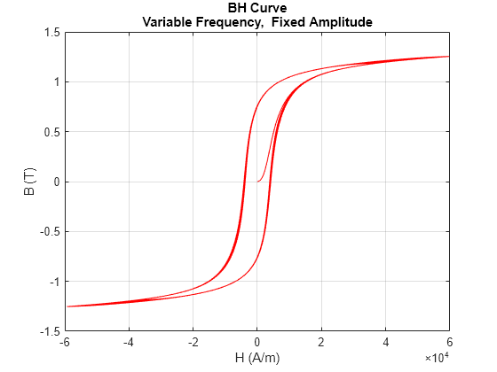
Set up the model to simulate without eddy losses and have a variable frequency and fixed amplitude magnetic field intensity input. Plot the B-H curve.

modelHysteresisEddyTransformerLossesPlotBHCurve(myModel,Amplitude="Variable",Frequency="Variable",ModelEddyLosses="false")

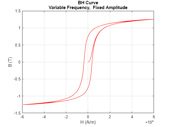
For a magnetic field intensity with a fixed amplitude, the B-H curve is independent of frequency. You can see this independence because the curves for magnetization cycles at different frequencies overlap. The hysteresis losses are proportional to the area inside the B-H curve and to the frequency of the input signal. The input signal is a chirp signal in which the frequency increases linearly with the simulation time. Therefore, the hysteresis losses must also increase approximately linearly with the simulation time. Plot the hysteresis losses over time to verify this increase.

modelHysteresisEddyTransformerLossesPlotLosses

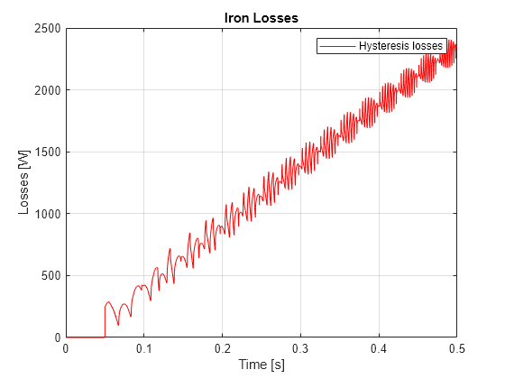
The energy is zero until 5e-2 s, which is the averaging period for hysteresis losses. When the block starts averaging the losses, the hysteresis losses increase linearly with the frequency.

Model Eddy Losses

Increase the Thickness of laminations parameter so the eddy losses are significant.

laminationThickness = 1.2; % mm

Set up the model to simulate both hysteresis and eddy current losses and have a variable frequency and a fixed amplitude magnetic field intensity input. Plot the B-H curve.

modelHysteresisEddyTransformerLossesPlotBHCurve(myModel,Amplitude="Fixed",Frequency="Variable",ModelEddyLosses="true")

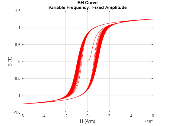
For a fixed amplitude, the curve does not overlap when the frequency increases. The curve becomes wider with the frequency. Given the increase in frequency and the area inside the curve, the eddy losses must increase faster than linearly with the frequency of the magnetization cycle. Plot the hysteresis and eddy current losses to verify this.

modelHysteresisEddyTransformerLossesPlotLosses

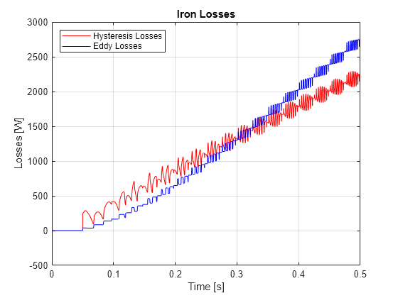
The software counts the hysteresis and eddy current losses after the first averaging period. The eddy losses are smaller than the hysteresis losses at low frequencies, but they increase faster with frequency.

Reduce Eddy Losses

You can avoid eddy current losses by laminating the iron core of transformers. Decrease the Thickness of laminations parameter and then plot the B-H curve and the eddy losses over time.

laminationThickness = 0.3; % [mm]
modelHysteresisEddyTransformerLossesPlotBHCurve(myModel,Amplitude="Fixed",Frequency="Variable",ModelEddyLosses="true")

modelHysteresisEddyTransformerLossesPlotLosses

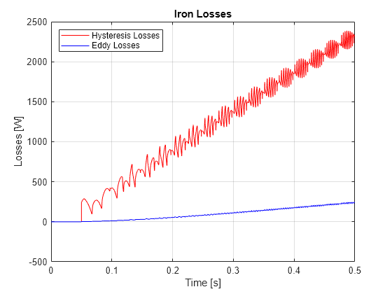
With thinner laminations, the B-H curve is not as wide and the eddy losses grow at a slower rate.