User-Defined Nonlinear Amplifier Model
This example shows how to:
Generate user-defined custom models by creating an RF Toolbox™ object in the MATLAB® workspace and importing it into an Equivalent Baseband amplifier block.
Create a nonlinear amplifier with an adjustable Pin-Pout curve.
Simulate intermodulation products in a two-tone test model.
In the example, the Vin-Vout relationship for the amplifier is a simple polynomial. The example uses this voltage relationship to generate a Pin-Pout curve that is incorporated into the amplifier model. Although the example uses a specific polynomial function, the same approach can be used to create arbitrary functions of power out and phase versus power in and frequency. Indeed, it can be used to set any of the writable properties of a component, such as S-parameters or noise properties.
Define the Voltage-Out Versus Voltage-In Relationship
Use MATLAB commands to create a vector of polynomial coefficients that define the desired Vin-Vout relationship. A MATLAB convention is to store nth order polynomial coefficients in a row vector of length n+1 with the nth power in the first element and the zeroth power (constant) in the last (n+1 th) element. The power series here is for illustration, and can easily be altered. You may recognize the values as the first twelve terms of the polynomial series expansion of the hyperbolic tangent function.
TanhSeries = [-1382/155925 0 62/2835 0 -17/315 0 2/15 0 -1/3 0 1 0];
Next choose a range for the independent variable, Vin, and define a vector of input voltage values over this range. The low end (1 mV here) should be sufficiently low that the linear term dominates Vout. The high end should be chosen such that Vout just reaches its local maximum value. The resulting Vout will be extrapolated for all Vin greater than 1.23. Next compute the vector of output voltage values, Vout, using the power series.
Vin = linspace(0.001,1.23,100);     % volts
Vout = polyval(TanhSeries, Vin);    % volts
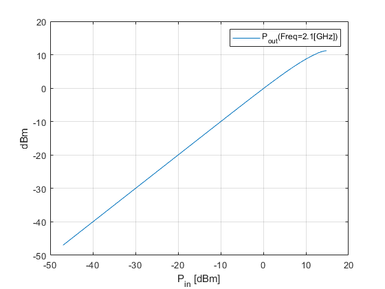
Create a Nonlinear Amplifier and Generate the Pin-Pout Curve
Create an RF Toolbox amplifier object with the default property values. Then, generate the Pin-Pout data (in watts) for the amplifier by dividing the square of the input and output voltage vectors by the reference impedance of the amplifier. Use the Pin-Pout data to specify the nonlinearity of the amplifier object. For this example, the Pin-Pout curve is defined for one frequency point (2.1 GHz) and used (by extrapolation) at all frequency points. See the RF Toolbox documentation for information on how to create a component with separately defined curves for any number of frequency points.
amp = rfckt.amplifier;
amp.NonlinearData.Freq = 2.1e9;             % Hz
Zref = 50;                                  % ohm
amp.NonlinearData.Pin  = {(Vin.^2)./Zref};  % watts
amp.NonlinearData.Pout = {(Vout.^2)./Zref}; % watts
In this example, we define the phase change to be zero for all Pin and all frequencies, but RF Toolbox lets you set it to be a function of Pin and frequency.
amp.NonlinearData.Phase = {zeros(size(Vin))};
Make the Small-Signal Gain Consistent with the Power Gain Slope at Low Power
Define the S21 parameter of the amplifier at the frequency point for which you specified the power data. The S21 network parameter must be consistent with the gain slope at the low power end of the Pin-Pout curve at that frequency point. If these values are inconsistent, RF Blockset software will attempt to reconcile the data and issue a warning that is has done so. To ensure consistency, define the S21 parameter to be the linear term of the power series that defines the Vin-Vout relationship. The linear term is the next-to-last element in the vector. Plot the Pin-Pout curve.
amp.NetworkData.Freq = amp.NonlinearData.Freq;
amp.NetworkData.Data = [0 0; TanhSeries(end-1) 0];
fig = figure;
plot(amp,'Pout');
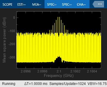
Run the Test Harness with an Input Power of 7 dBm per Tone
The following figure shows the test harness for your new amplifier. The input signal consists of the sum of two tones, one 10kHz below the center frequency, and one 10kHz above it. The spectrum scope shows the various intermodulation products at higher and lower frequencies than the two test tones. The EVM subsystem calculates error vector magnitude. Open and Run "rfb_user_defined_amp_mdl" model. To view and edit the preset model workspace values, click the Modeling Tab in the Toolstrip and select Model Explorer.
%

open('rfb_user_defined_amp_mdl.slx');

sim('rfb_user_defined_amp_mdl');
Rerun the Simulation Using an Input Power Level of 8 dBm per Tone
To increase the source power from 7dBm to 8 dBm from a MATLAB script, first get the handle to the current Simulink® model workspace. Then set the appropriate workspace variable (power_in_dBm in this example) to the value 8. Rerun the simulation. Notice that 11th order intermods (outermost tones on the spectrum scope) increase by about 11 dB.
hws=get_param(bdroot, 'modelworkspace');
hws.assignin('power_in_dBm', 8);
sim('rfb_user_defined_amp_mdl');
Truncate the Hyperbolic Tangent Series to Only the First Four Terms
Reset the input power to 7 dBm. Then, specify the power series for the hyperbolic tangent using only the first four terms of the series. Recalculate the output voltage values and the amplifier Pin-Pout data. Rerun the simulation. The spectrum scope shows that only the third intermodulation products are produced. You can also set the stop time to inf, rerun the simulation, and experiment to see the effect of the slider gain (Blue box on the Simulink model).
hws.assignin('power_in_dBm', 7);
TanhSeries = [-1/3 0 1 0];
Vin = linspace(0.001,1,100);                % volts
Vout = polyval(TanhSeries, Vin);            % volts
amp.NonlinearData.Pin  = {(Vin.^2)./Zref};  % watts
amp.NonlinearData.Pout = {(Vout.^2)./Zref}; % watts
sim('rfb_user_defined_amp_mdl');
bdclose('rfb_user_defined_amp_mdl');
close(fig);
See Also
Output Port | <docid:simrf_ref#f1-627147> | <docid:simrf_ref#bvflpaq> | <docid:rf_ref#mw_c074a0c8-70fc-48fa-820c-1873b5a8f2ce>