Model Lossy Transmission Lines in Parallel Link Designer

The Parallel Link Designer app uses a frequency dependent RLGC model to represent a lossy transmission line model. The app uses a 2-D field solver with a transmission line editor. Using the transmission line editor, you can enter the cross-section of different model types. You can also directly define a table-driven loss model in IsSpice4.

Types of Lossy Transmission Line Models

Single Conductor and Differential Lossy Transmission Line Models

You can create single conductor and differential lossy transmission line models for these model types:

• Simple lossy transmission line

• Microstrip

• Buried microstrip

• Stripline

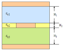
The parameters in each model type define the relationship of the physical geometries for the transmission line model. You can also define etch shape and enable tabbed routing.

If you need to combine multiple dielectrics in the actual physical stackup in a single dielectric in the editor, combine them by their proportional thickness. For example, for a stripline with three dielectrics, the single ε_r is:

$${\epsilon }_r=\frac{{\epsilon }_{r1}{\text{H}}_{\text{1}}+{\epsilon }_{r2}{\text{H}}_{\text{2}}+{\epsilon }_{r3}{\text{H}}_{\text{3}}}{{\text{H}}_{\text{1}}{\text{+H}}_{\text{2}}{\text{+H}}_{\text{3}}}$$

Coupled Lossy Transmission Line Model Types

You can create single-ended and differential coupled lossy transmission line models for these model types:

• Microstrip

• Buried microstrip

• Stripline

To create a coupled model, you have to enable the parameter Coupled and set the parameter Aggressor to an integer value in the Lossy Transmission Line Editor dialog box. For single conductors, set the aggressor value between 1 and 20. For differential conductors, set the aggressor value between 1 and 9.

Analytical RLGC Model

Formulating Single-Line Models

For single-line case, the parameters R, L, G, and C are scalar.

From Telegrapher's equation:

$$\begin{array}{l}\frac{\partial V}{\partial x}=-RI-2\pi fLI\\ \frac{\partial I}{\partial x}=-GV-2\pi fCV\end{array}$$

The solution to the coupled partial differential equations results in two waves travelling in opposite directions along the x-axis. The solution can be written as:

$$\begin{array}{l}{Y}_{0}V=W_{+}{e}^{-\gamma x}+W_{-}{e}^{-\gamma (l-x)}\\ I=W_{+}{e}^{-\gamma x}-W_{-}{e}^{-\gamma (l-x)}\end{array}$$

where $$Y_0\equiv \sqrt{\frac{G+2\pi fC}{R+2\pi fL}}$$, $$\gamma \equiv \sqrt{(G+2\pi fC)(R+2\pi fL)}$$ and l is the length of the transmission line.

Evaluate these equations at boundary conditions x=0 and x=l and set $$X_d\equiv e^{-\gamma l}$$:

$$\begin{array}{l}{Y}_{0}V(0)=W_{+}+X_d{W}_{-}\\ Y_{0}V(l)=W_{-}+X_d{W}_{+}\\ I(0)=W_{+}-X_d{W}_{-}\\ I(l)=W_{-}-X_d{W}_{+}\end{array}$$

Convert the frequency domain equations to time domain to perform transient analysis in SPICE:

$$\begin{array}{l}{Y}_0\ast V(0,t)=W_{+}(t)+X_d\ast W_{-}(t)\\ Y_0\ast V(l,t)=W_{-}(t)+X_d\ast W_{+}(t)\\ I(0,t)=W_{+}(t)-X_d\ast W_{-}(t)\\ I(l,t)=W_{-}(t)-X_d\ast W_{+}(t)\end{array}$$

Here, W₊(t) is the wave that launches from the x=0 end of the transmission line and travels towards the x=l end. Similarly, W_-(t) is the wave that launches from the x=l end of the transmission line and travels towards the x=0 end.

Solve for W₊(t) and W_-(t):

$$W_{+}(t)=\frac{1}{2}\left(Y_0\ast V(0,t)+I(0,t)\right)$$

$$W_{-}(t)=\frac{1}{2}\left(Y_0\ast V(l,t)+I(l,t)\right)$$

Multi-Conductor Line

For multi-conductor line case, the parameters R, L, G, and C are appropriately sized symmetric positive-definite matrices. Using the sqrtm and mldivide functions to find the square root and division results, the equations for Y₀ and γ becomes:

γ=sqrtm(G+2πfC)(R+2πfL)

and

Y0=γ\(G+2πfC)

And using the expm to find the exponential, the equation for X_d becomes:

Xd=expm(-γl)

These equations support the single line case, the symmetric two-line case, and the multiple line structure that comes from a uniform dielectric. But in general, the modes change with frequency. So removing the delay according to the high-frequency mode shape leads to ripples in the high-frequency response.

Table-Driven Loss Model

The analytical RLGC model converts the input data to an internal table of loss vs. frequency. This internal table is used to calculate the lossy transmission line model. However, a real world table data often contains causality violations. The algorithm needs to detect and correct these violations to develop a successful model.

For the overall transmission line to be causal, both the impedance per unit length (Z) and (Y) need to be causal. The algorithm uses the rational function if to detect and fix the causality problems. But if the table has few data points or if the discontinuities are too strong, the algorithm estimates the asymptotes of the data points and treat them as analytical model.

Example Lossy Transmission Line Model Based on Loss Table

.model example_table_model W MODELTYPE=table N=2 RMODEL=r_ex1
+ LMODEL=l_ex1 GMODEL=g_ex1 CMODEL=c_ex1
* Example usage:
* W1 1 2 0 3 4 0 N=2 L=<length> TABLEMODEL=ex1
.model r_ex1 sp N=2 SPACING=nonuniform VALTYPE=real
+ INTERPOLATION=spline
+ DATA = 161
+ 0          
+        2.830786883265845
+       0.9435956277553057
+        2.830786883265899
+ 5e+007      
+        7.984518593654459
+        2.725935368837102
+        7.985009453309226
+ 1e+008      
+        11.31284926513239
+        3.874158264111289
+        11.31305325358019
+ 1.5e+008    
+        13.98304266450885
+        4.795464684133719
+        13.98145490109022
+ 2e+008      
+         16.1812358691131
+        5.552866396931773
+        16.17606159366768
+ 2.5e+008    
+        18.09223128657047
+        6.210205279801264
+        18.08227217758706
+ 3e+008      
+        19.82023821675704
+        6.803816219431784
+        19.80497533258797
+ 3.5e+008    
+        21.41863053348143
+        7.352397271135547
+        21.39796746108365
...

Editing Lossy Conductor Line Models

You can edit lossy transmission lines and coupled models for pre-layout analysis using the Lossy Transmission Line Editor dialog box. There are two modes for editing or creating models using the Lossy Transmission Line Editor dialog box:

• Standalone library mode — Quickly create and edit different types of lossy models and store them in a library location. You can create a common library directory and access the model from multiple projects. You can also reuse the models across different designs by copying them and pasting them in the new design. If you edit any model in the common library, the changes in the model appear in all the projects where the model is used.

  To access the dialog box, select Tools > Lossy Transmission Line Editor from the app toolstrip.

• Interactive mode — Interactively use the Lossy Transmission Line Editor in the schematic to create and edit lossy models and coupled models on the fly for a selected transmission line. To access the editor, right click on the w-line element symbol in the schematic and select Edit T-line Properties.

Related Topics

• Loss in Transmission Line Corners