Simulate and Mitigate FMCW Interference Between Automotive Radars
This example shows how to simulate frequency-modulated continuous-wave (FMCW) interference between two multiple input multiple output (MIMO) automotive radars in a highway driving scenario. Missed and ghost targets caused by interferences are simulated and visualized. This example also applies spatial-domain interference mitigation and shows the interference mitigation result.
Introduction
With the increasing number of vehicles being equipped with multiple radars in automotive scenarios, interference detection and mitigation have become essential for automotive radars. Interference can affect the functionality of radar systems in many different ways. Interference can increase the noise level of the range-angle-Doppler map and decrease the probability of detection. The signal to interference and noise ratio (SINR) depends on the distance and angles separating two radars, as well as radar parameters such as antenna gain, antenna transmit power, array size, bandwidth, center frequency, and chirp duration. Low SINR results in missed detections for low radar cross section (RCS) targets, creating a blind spot in some regions. Another challenge with radar interference is ghost targets, in which the radar detects an object that doesn't exist. The victim radar can mitigate interference by fast-time/slow-time domain interference removal/signal reconstruction, spatial-domain beamforming/detector design, etc.
Waveform and Transceiver Definitions
Define Victim Baseband FMCW Radar Waveform
The victim radar is designed to use an FMCW waveform which is a common waveform in automotive applications because it enables range and Doppler estimation through computationally efficient fast Fourier transform (FFT) operations. For illustration purposes, in this example, configure the radar to a maximum range of 150 m. The victim radar operates at a 77 GHz frequency. The radar is required to resolve objects that are at least 1 meter apart. Because this is a forward-facing radar application, the maximum relative speed of vehicles on highway is specified as 230 km/h.
rng(2023);             % Set random number generator for repeatable results
fc = 77e9;             % Center frequency (Hz)
c = physconst('LightSpeed');             % Speed of light (m/s)
lambda = freq2wavelen(fc,c);             % Wavelength (m)
rangeMax = 150;        % Maximum range (m)
rangeRes = 1;          % Desired range resolution (m)
vMax = 230*1000/3600;  % Maximum relative velocity of cars (m/s)
fmcwwav1 = helperFMCWWaveform(fc,rangeMax,rangeRes,vMax);
sig = fmcwwav1();
Ns = numel(sig);
Define Interfering Baseband FMCW Radar Waveform
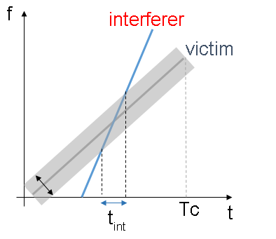
Consider an interfering radar using FMCW modulation. The frequency spectrum characteristics of the interference in the victim radar depend on the chirp's relative timing and slopes.
fcRdr2 = 77e9;         % Center frequency (Hz)
lambdaRdr2 = freq2wavelen(fcRdr2,c);              % Wavelength (m)
rangeMaxRdr2 = 100;    % Maximum range (m)
rangeResRdr2 = 0.8;     % Desired range resolution (m)
vMaxRdr2 = vMax;       % Maximum Velocity of cars (m/s)
fmcwwav2 = helperFMCWWaveform(fcRdr2,rangeMaxRdr2,rangeResRdr2,vMaxRdr2);
sigRdr2 = fmcwwav2();
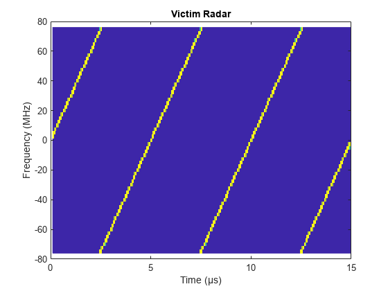
Plot the victim radar baseband waveform in the first 3 pulses.
figure
pspectrum(repmat(sig,3,1),fmcwwav1.SampleRate,'spectrogram', ...
    'Reassign',true,'FrequencyResolution',10e6)
axis([0 15 -80 80]); title('Victim Radar'); colorbar off
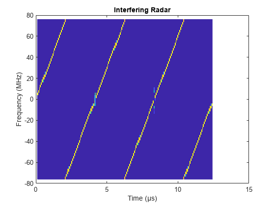
Plot the interfering radar baseband waveform with steeper chirp slopes in the first 3 pulses.
figure
pspectrum(repmat(sigRdr2,3,1),fmcwwav1.SampleRate,'spectrogram',...
    'Reassign',true,'FrequencyResolution',10e6,'MinThreshold',-13)
axis([0 15 -80 80]); title('Interfering Radar'); colorbar off;
Model Victim and Interfering MIMO Radar Transceivers
Consider both radars use a uniform linear array (ULA) to transmit and use a ULA to receive the radar waveforms. Using a receive array enables the radar to estimate the azimuthal direction of the reflected energy received from potential targets. Using a transmit array enables the radar to form a large virtual array at the receiver to improve the azimuthal angle resolution. To receive the target and noise signals at the victim radar, model the victim radar's monostatic transceiver using radarTransceiver and specifying the transmit and receive ULAs of the victim radar in its properties.
% Set radar basic transceiver parameters
antAperture = 6.06e-4;                          % Antenna aperture (m^2)
antGain = aperture2gain(antAperture,lambda);    % Antenna gain (dB)
txPkPower = db2pow(13)*1e-3;                    % Tx peak power (W)
rxNF = 4.5;                                     % Receiver noise figure (dB)

% Construct the receive array for victim radar
Nvr =  16;     % Number of receive elements for victim radar
vrxEleSpacing = lambda/2;        % Receive element spacing for victim radar
antElmnt = phased.IsotropicAntennaElement('BackBaffled',false);
vrxArray = phased.ULA('Element',antElmnt,'NumElements',Nvr,...
    'ElementSpacing',vrxEleSpacing);

% Construct the transmit array for victim radar
Nvt = 2;     % Number of transmit elements for victim radar
vtxEleSpacing = Nvr*vrxEleSpacing;     % Transmit element spacing for victim radar
vtxArray = phased.ULA('Element',antElmnt,'NumElements',Nvt,...
    'ElementSpacing',vtxEleSpacing);

% Model victim radar monostatic transceiver for receiving target and noise
% signals
vradar = radarTransceiver("Waveform",fmcwwav1,'ElectronicScanMode','Custom');
vradar.Transmitter = phased.Transmitter('PeakPower',txPkPower,'Gain',antGain);
vradar.TransmitAntenna = phased.Radiator('Sensor',vtxArray,'OperatingFrequency',fc,'WeightsInputPort',true);
vradar.ReceiveAntenna = phased.Collector('Sensor',vrxArray,'OperatingFrequency',fc);
vradar.Receiver = phased.ReceiverPreamp('Gain',antGain,'NoiseFigure',rxNF,'SampleRate',fmcwwav1.SampleRate);
Different from the target signals, the interference is transmitted from the transmit ULA of the interfering radar and received by the receive ULA of the victim radar. Model the interference transceiver using the helperInterferenceTransceiver function, which includes the transmit ULA of the interfering radar and the receive ULA of the victim radar in its inputs.
% Construct the transmit array for interfering radar
Nit = 3;     % Number of transmit elements for interfering radar
Nir = 4;     % Number of receive elements for interfering radar
irxEleSpacing = lambda/2;        % Receive element spacing for interfering radar
itxEleSpacing = Nir*irxEleSpacing;     % Transmit element spacing for interfering radar
itxArray = phased.ULA('Element',antElmnt,'NumElements',Nit,...
    'ElementSpacing',itxEleSpacing);

% Model interference transceiver for receiving interference signal at the
% victim radar
iradar = helperInterferenceTransceiver(fmcwwav2,txPkPower,antGain,fc,itxArray,vrxArray);
Simulate Driving Scenario
Create a highway driving scenario with two vehicles traveling in the vicinity of the ego vehicle with a forward-facing victim radar. The vehicles are modeled as cuboids and have different velocities and positions defined in the driving scenario. The ego vehicle is moving with a velocity of 25 m/s, the target vehicle is moving at 34 m/s in the same direction, and the interfering vehicle with a forward-facing interfering radar is moving at -50 m/s in the opposite direction. For details on modeling a driving scenario, see the example Create Actor and Vehicle Trajectories Programmatically (Automated Driving Toolbox). The radar sensor is mounted on the front of the ego and interfering vehicles.
To create the driving scenario, use the helperAutoDrivingScenario function. To examine the contents of this function, use the edit('helperAutoDrivingScenario') command.
% Create driving scenario
[scenario, egoCar] = helperAutoDrivingScenario;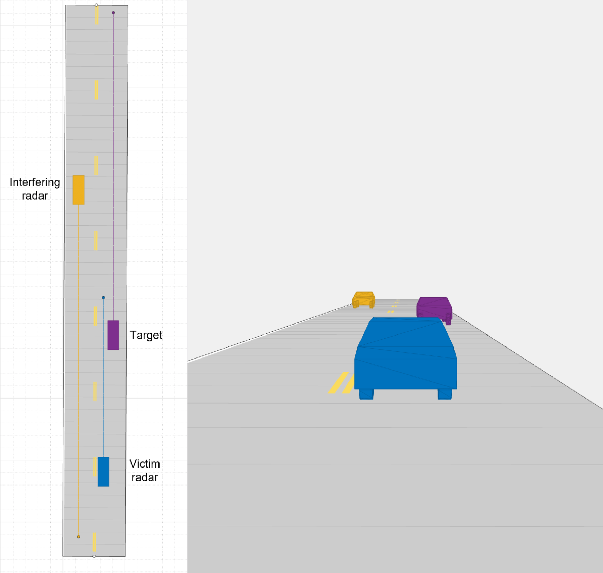
To visualize and modify the driving scenario, use the drivingScenarioDesigner with the current scenario as the input:
drivingScenarioDesigner(scenario)
Use the following code to see the initial ranges, angles and velocities of the target vehicle and the interfering vehicle relative to the ego vehicle. The leaving target vehicle is located at 22.0 m and -4.2 degrees at a velocity of 9.0 m/s relative to the victim radar, and the coming interfering vehicle on the opposite direction is located at 48.3 m and 4.8 degrees at a velocity of -74.7 m/s relative to the victim radar.
% Initialize target poses in ego vehicle's reference frame
tgtPoses = targetPoses(egoCar);

% Target vehicle's range and angle relative to the victim radar
[tarRange,tarAngle] =  rangeangle(tgtPoses(1).Position');

% Target vehicle's radial velocity relative to the victim radar (the negative sign is due to different reference axes in radialspeed and drivingScenarioDesigner)
tarVelocity = -radialspeed(tgtPoses(1).Position',tgtPoses(1).Velocity');

% Interfering vehicle's range and angle relative to the victim radar
[intRange,intAngle] =  rangeangle(tgtPoses(2).Position');

% Interfering vehicle's radial velocity relative to the victim radar
intVelocity = -radialspeed(tgtPoses(2).Position',tgtPoses(2).Velocity');
Transceiver Signal Processing
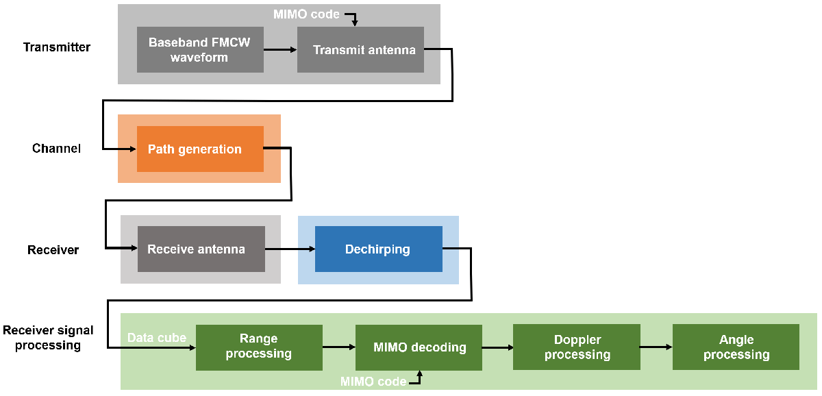
To form a large virtual array at the MIMO radar receiver, the transmit waveforms on different transmit antennas need to be orthogonal such that the receiver can separate signals from different transmit antennas. This example adopts time division multiplexing (TDM) to achieve the waveform orthogonality. In each pulse, a vector of TDM-MIMO code is weighted on the transmit array. For the principle on virtual array and TDM-MIMO radar, see the example Increasing Angular Resolution with Virtual Arrays.
The radar collects a train of the pulses of the FMCW waveform at each of the receive ULA antenna elements. These collected pulses on different receive antennas form a data cube, which is defined in Radar Data Cube. The data cube is coherently processed along the fast-time, slow-time, and array dimensions to estimate the range, Doppler and angle of potential targets.
The overall transceiver signal processing workflow for a MIMO radar is summarized below. The gray blocks are implemented using radarTransceiver with the channel paths and the TDM-MIMO code in its inputs. The path generation block generates the two-way target path, the one-way interference path, and the interference multipath. The green blocks show the data cube processing flow for MIMO radar.
Obtain Interference-free and Interfered Data Cubes
The following code generates the received interference pulse train at the victim radar. For victim radar to dechirp interference in each of its pulse, the received interference pulse train is parsed according to the victim radar's frame structure, such that the number of fast-time samples in each parsed interference pulse is equal to the number of fast-time samples of the victim radar Nft.
% Define fast-time and slow-time samples
Nft = round(fmcwwav1.SweepTime*fmcwwav1.SampleRate);  % Number of fast-time samples of victim radar
Nsweep = 192;                                         % Number of slow-time samples of victim radar
Nift = round(fmcwwav2.SweepTime*fmcwwav2.SampleRate); % Number of fast-time samples of interfering radar
Nisweep = ceil(Nft*Nsweep/Nift);                      % Number of slow-time samples of interfering radar

% Generate TDM-MIMO code for interfering antenna elements
wi = helperTDMMIMOEncoder(Nit,Nisweep);

% Assemble interference pulse train at interfering radar's scenario time
rxIntTrain = zeros(Nift*Nisweep,Nvr);

% Initialize scenario time
time = scenario.SimulationTime;

% Initialize actor profiles
actProf = actorProfiles(scenario);

% Get interference pulse train at interfering radar's scenario time
for l = 1:Nisweep
    % Generate all paths to victim radar
    ipaths = helperGenerateIntPaths(tgtPoses,actProf,lambdaRdr2);

    % Get the received signal with interference only
    rxInt = iradar(ipaths,time,wi(:,l));
    rxIntTrain((l-1)*Nift+1:l*Nift,:) = rxInt;

    % Get the current scenario time
    time = time + fmcwwav2.SweepTime;

    % Move targets forward in time for next sweep
    tgtPoses(1).Position=[tgtPoses(1).Position]+[tgtPoses(1).Velocity]*fmcwwav2.SweepTime;
    tgtPoses(2).Position=[tgtPoses(2).Position]+[tgtPoses(2).Velocity]*fmcwwav2.SweepTime;
end

% Truncate interference pulse train to the length of target pulse train
rxIntTrain = rxIntTrain(1:Nft*Nsweep,:);

% Assemble interference pulse train at victim radar's scenario time
rxIntvTrain = permute(reshape(rxIntTrain,Nft,Nsweep,Nvr),[1,3,2]);
Dechirp the target signal at the victim radar to obtain the interference-free data cube, which is used to plot the target response as an ideal performance baseline. Also, dechirp the combined target and interference signal to obtain the interfered data cube, which is used to plot interference effects on target detection.
% Generate TDM-MIMO code for victim antenna elements
wv = helperTDMMIMOEncoder(Nvt,Nsweep);

% Assemble interference-free data cube
XcubeTgt = zeros(Nft,Nvr,Nsweep);

% Assemble interfered data cube
Xcube = zeros(Nft,Nvr,Nsweep);

% Initialize scenario time
time = scenario.SimulationTime;

% Initialize target poses in ego vehicle's reference frame
tgtPoses = targetPoses(egoCar);

% Initialize actor profiles
actProf = actorProfiles(scenario);

% Get data cube at victim radar's scenario time
for l = 1:Nsweep
    % Generate target paths to victim radar
    vpaths = helperGenerateTgtPaths(tgtPoses,actProf,lambda);

    % Get the received signal without interference
    rxVictim = vradar(vpaths,time,wv(:,l));

    % Dechirp the interference-free target signal
    rxVsig = dechirp(rxVictim,sig);

    % Save sweep to data cube
    XcubeTgt(:,:,l) = rxVsig;

    % Get the received interference signal
    rxInt = rxIntvTrain(:,:,l);

    % Dechirp the interfered signal
    rx = dechirp(rxInt+rxVictim,sig);
    Xcube(:,:,l) = rx;

    % Get the current scenario time
    time = time + fmcwwav1.SweepTime;

    % Move targets forward in time for next sweep
    tgtPoses(1).Position=[tgtPoses(1).Position]+[tgtPoses(1).Velocity]*fmcwwav1.SweepTime;
    tgtPoses(2).Position=[tgtPoses(2).Position]+[tgtPoses(2).Velocity]*fmcwwav1.SweepTime;
end
Receiver Signal Processing on Interference-free Data Cube
Use the phased.RangeResponse object to perform the range processing on the interference-free radar data cubes. Use a Hann window to suppress the large sidelobes produced by the vehicles when they are close to the radar.
% Calculate number of range samples
Nrange = 2^nextpow2(Nft);

% Define range response
rngresp = phased.RangeResponse('RangeMethod','FFT', ...
    'SweepSlope',fmcwwav1.SweepBandwidth/fmcwwav1.SweepTime, ...
    'RangeFFTLengthSource','Property','RangeFFTLength',Nrange, ...
    'RangeWindow','Hann','SampleRate',fmcwwav1.SampleRate);

% Calculate the range response of interference-free data cube
XrngTgt = rngresp(XcubeTgt);
The victim radar decodes TDM-MIMO radar waveform by separating the Nvt TDM-MIMO transmit waveforms at each of its Nrt receive chains to form a virtual array of size Nv. After the waveform separation, the victim radar applies Doppler FFT on pulses for each range bin and virtual array element.
% Decode TDM-MIMO waveform
[XdecTgt,Nsweep] = helperTDMMIMODecoder(XrngTgt,wv);

% Number of Doppler samples
Ndoppler = 2^nextpow2(Nsweep);

% Size of virtual array
Nv = Nvr*Nvt;

% Doppler FFT with Hann window
XrngdopTgt = helperVelocityResp(XdecTgt,Nrange,Nv,Ndoppler);
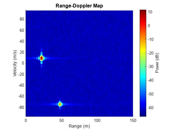
Next, plot the range-Doppler map for the interference-free case. The range-Doppler map only shows the velocity from negative maximum unambiguous velocity to positive maximum unambiguous velocity. The maximum unambiguous velocity is inversely proportional to the pulse repetition interval on each transmit antenna elements. The range-Doppler map below shows that the target vehicle is located at near 22.0 m at a velocity of near 9.1 m/s and the interfering vehicle is located at near 47.6 m at a velocity of near -74.5 m/s.
% Pulse repetition interval for TDM-MIMO radar
tpri = fmcwwav1.SweepTime*Nvt;

% Maximum unambiguous velocity
vmaxunambg = lambda/4/tpri;

% Plot range-Doppler map
helperRangeVelocityMapPlot(XrngdopTgt,rngresp.SweepSlope,...
    fmcwwav1.SampleRate,tpri,rangeMax,vmaxunambg,Nrange,Ndoppler,lambda);
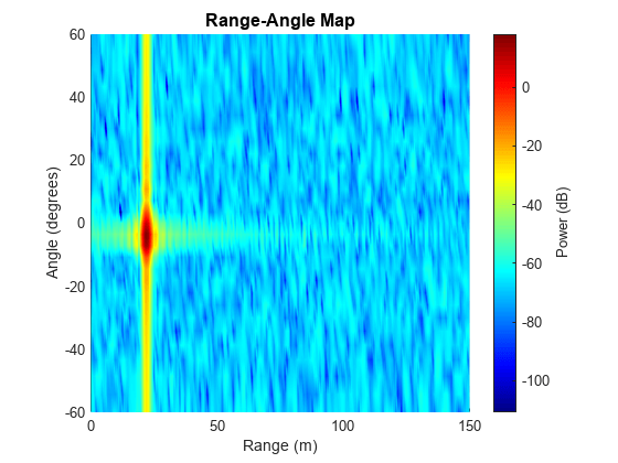
Apply angle FFT on virtual array at each range-Doppler bin for angle estimation. At the target's Doppler bin, the signal of the target vehicle is coherently integrated in the Doppler domain while the signal of the interfering vehicle with another velocity is not coherently integrated. Thus, in the range-angle map at the target's Doppler bin, the coherently integrated target's peak is strong. The range-angle map below shows that the target is located near 22.0 m and -3.6 degrees.
% Number of angle samples
Nangle = 2^nextpow2(Nv);

% Angle FFT with Hann window
XrngangdopTgt = helperAngleResp(XrngdopTgt,Nrange,Nangle,Ndoppler);

% Target Doppler bin
tarDopplerBin = ceil(tarVelocity/lambda*2*tpri*Ndoppler+Ndoppler/2);

% Plot range-angle map
helperRangeAngleMapPlot(XrngangdopTgt,rngresp.SweepSlope,...
    fmcwwav1.SampleRate,rangeMax,vrxEleSpacing,Nrange,Nangle,tarDopplerBin,lambda);
Receiver Signal Processing on Interfered Data Cube
Apply the same receiver signal processing workflow to the interfered data cube.
% Calculate the range response of interfered data cube
Xrng = rngresp(Xcube);

% Decode TDM-MIMO waveform
[Xdec,Nsweep] = helperTDMMIMODecoder(Xrng,wv);

% Velocity FFT with Hann window
Xrngdop = helperVelocityResp(Xdec,Nrange,Nv,Ndoppler);
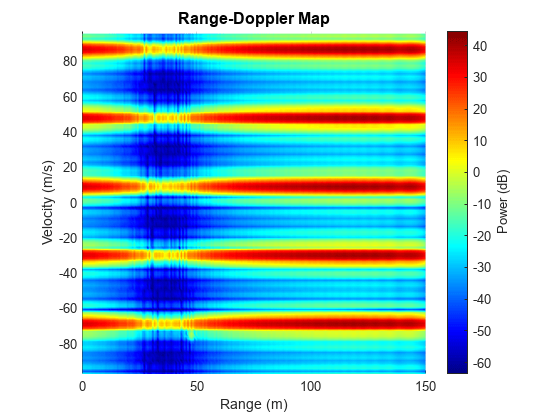
Plot range-Doppler map of the interfered data cube. We can see the strong interference is a wideband signal that occupies a large number of range bins and hides the peaks of the two vehicles.
% Plot range-Doppler map
helperRangeVelocityMapPlot(Xrngdop,rngresp.SweepSlope,...
    fmcwwav1.SampleRate,tpri,rangeMax,vmaxunambg,Nrange,Ndoppler,lambda);
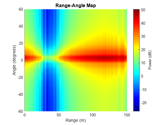
Plot range-angle map of the interfered data cube at the target's Doppler bin. We can see the strong interference raises the noise floor and hides the peak of the target. We can also observe that the interference angle of arrival is near 3.6 degrees.
% Angle FFT with Hann window
Xrngangdop = helperAngleResp(Xrngdop,Nrange,Nangle,Ndoppler);

% Plot range-angle map of range-angle FFT
[angGrid,rangeGrid] = helperRangeAngleMapPlot(Xrngangdop,rngresp.SweepSlope,...
    fmcwwav1.SampleRate,rangeMax,vrxEleSpacing,Nrange,Nangle,tarDopplerBin,lambda);
Interference Effect Animation
The following animation shows the interference effects for FMCW radars with different waveform parameters for the interfering radar. In this example, the bandwidth for both radars is set to be 150.0 MHz, the chirp duration for the victim radar is considered to be 5.0 μs, and the chirp duration for the interfering radar is changed from 2.0 μs to 5.0 μs with a step size of 0.33 μs. We can observe that when the chirp duration of the interfering radar changes, the range-Doppler map also changes. If the interference chirp slope is the same as the victim radar's chirp slope, point-like ghost targets may appear in the range-Doppler map. If the strong interference or its sidelobe is overlapped with the target on the target's range-Doppler bin, in the range-angle map, we can observe the interference angle of arrival and may observe the missing of the target due to the high noise level elevation caused by the direct-path interference.

Spatial-Domain Interference Mitigation
Interference can be mitigated by fast-time/slow-time domain interference removal/signal reconstruction, spatial-domain beamforming/detector design, etc. This example shows how to mitigate interference in spatial-domain using phased.GLRTDetector.
Post range-Doppler FFT, the received spatial-domain signal on virtual array can be modeled as
,
where is the desired target's complex amplitude, is spatial-domain noise on the virtual array, is the Kronecker product, and are target receive and transmit steering vectors, is interference receive steering vector with same length as , and is decoded interference transmit steering vector with same length as . As the interferer's transmit array configurations, MIMO codes, and FMCW parameters are unknown at the victim radar, the decoded interference transmit steering vector is unknown. However, the interference receive steering vector only depends on the interference angle of arrival, which can be known or estimated when the victim radar passively senses the interference during its transmission idle period. This example assumes the perfect knowledge of interference receive steering vector.
% Configure receive steering vector using receive array of victim radar
vrxSv = phased.SteeringVector('SensorArray',vrxArray);

% Interference receive steering vector
iSv = vrxSv(fc,intAngle);
To apply the knowledge of interference receive steering vector in GLRT-based interference mitigation, the received spatial-domain signal on virtual array can be rewritten as
,
where is observation matrix, is the identity matrix, and includes unknown parameters. To test the existence of the desired target on multiple angles, the GLRT detector requires the input of multiple observation matrices with target virtual steering vectors sweeping at different directions.
% Configure virtual array
vArray = phased.ULA('Element',antElmnt,'NumElements',Nv,'ElementSpacing',vrxEleSpacing);

% Configure steering vector using virtual array of victim radar
vSv = phased.SteeringVector('SensorArray',vArray);

% Initialize observation matrix
obs = zeros(Nv,1+Nvt,Nangle);

% Obtain observation matrix for multiple angle bins
for angBin = 1:Nangle
    % Target virtual steering vector
    angGridSv = vSv(fc,angGrid(angBin));

    % Observation matrix for each angle bin
    obs(:,:,angBin) = [angGridSv,kron(eye(Nvt),iSv)];
end
The goal of the GLRT detection is to determine the existence of the desired target, which corresponds to the following hypothesis testing problem:
Rewritten this problem in terms of :
where is a row vector of zero with the same length as . Thus, the augmented hypothesis matrix inputted into GLRT detector is given below.
% Linear hypothesis
A = [1,zeros(1,Nvt)]; b = 0;

% Augmented hypothesis matrix
hyp = [A,b];
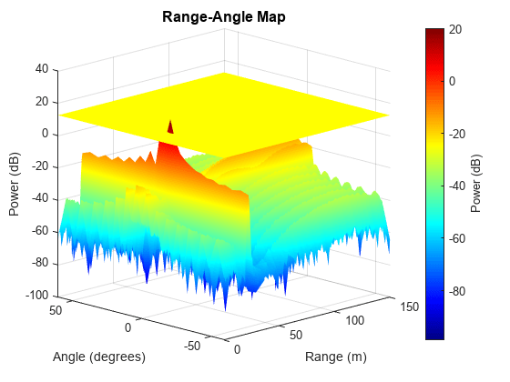
Obtain GLRT detection statistics on the received virtual array signal at the target's Doppler bin. Notice that the noise distribution may not be zero-mean due to the existence of MIMO decoding residual. Thus, avoid GLRT-based noise power estimation that assumes zero-mean white Gaussian noise, and estimate noise power from nearby range bins. Plot the GLRT detection statistics and detection threshold at the target's Doppler bin on the range-angle map and output the range-angle detection result.
% Configure GLRT detector
glrt = phased.GLRTDetector('ProbabilityFalseAlarm',1e-4,...
    'ThresholdOutputPort',true,'NoiseInputPort',true);

% Noise estimation from nearby range bins
noise = helperNoiseEstimator(Xrngdop,tarDopplerBin,Nv);

% Obtain GLRT detection statistics
[dresult,stat,th] = glrt(Xrngdop(:,:,tarDopplerBin)',hyp,obs,noise);

% Plot detection statistics and detection threshold on range-angle map
rngangResult = helperRangeAngleGLRTShowResult(dresult,stat,th,rangeMax,rangeGrid,angGrid)
rngangResult = 3×2

   21.2402   -3.5833
   21.9727   -3.5833
   22.7051   -3.5833
The range-angle map and detection result show that the target is located near 22.0 m and -3.6 degrees, and the interference is significantly mitigated.
Summary
This example shows how to generate a highway driving scenario with interfering radars using Automated Driving Toolbox. This example also shows how to model the FMCW interference for MIMO automotive radars using Radar Toolbox. This example demonstrates the phenomena of mutual automotive radar interference and shows the effectiveness of the GLRT detector for spatial-domain interference mitigation using Phased Array System Toolbox.
Reference
[1] M. Richards. Fundamentals of Radar Signal Processing. New York: McGraw Hill, 2005.
[2] Steven M. Kay, Fundamentals of Statistical Signal Processing: Detection Theory, Prentice Hall, 1998.
[3] S. Jin, P. Wang, P. Boufounos, P. V. Orlik, R. Takahashi and S. Roy, "Spatial-Domain Interference Mitigation for Slow-Time MIMO-FMCW Automotive Radar," 2022 IEEE 12th Sensor Array and Multichannel Signal Processing Workshop (SAM), 2022, pp. 311-315.
Helper Functions
helperFMCWWaveform Function
function fmcwwav = helperFMCWWaveform(fc,maxrange,rangeres,maxvel)
c = physconst('LightSpeed');                  % Speed of light in air (m/s)
lambda = freq2wavelen(fc,c);                  % Wavelength (m)

% Set the chirp duration to be 5 times the max range requirement
tm = 5*range2time(maxrange,c);                % Chirp duration (s)

% Determine the waveform bandwidth from the required range resolution
bw = rangeres2bw(rangeres,c);                 % Corresponding bandwidth (Hz)

% Set the sampling rate to satisfy both range and velocity requirements
sweepSlope = bw/tm;                           % FMCW sweep slope (Hz/s)
fbeatMax = range2beat(maxrange,sweepSlope,c); % Maximum beat frequency (Hz)
fdopMax = speed2dop(2*maxvel,lambda);         % Maximum Doppler shift (Hz)
fifMax = fbeatMax+fdopMax;                    % Maximum received IF (Hz)
fs = max(2*fifMax,bw);                        % Sampling rate (Hz)

% Configure the FMCW waveform using the waveform parameters derived from the requirements
fmcwwav = phased.FMCWWaveform('SweepTime',tm,'SweepBandwidth',bw,'SampleRate',fs,'SweepDirection','Up');
end
helperInterferenceTransceiver Function
function iradar = helperInterferenceTransceiver(waveform,txPkPower,antGain,fc,itxArray,vrxArray)
% Reuse radarTransceiver for transmitting interference signal at the
% interfering radar and receiving interference signal at the victim radar
iradar = radarTransceiver("Waveform",waveform,'ElectronicScanMode','Custom');

% Sepcify interfering radar transmitter
iradar.Transmitter = phased.Transmitter('PeakPower',txPkPower,'Gain',antGain);

% Sepcify transmit array as the interfering radar transmit array
iradar.TransmitAntenna = phased.Radiator('Sensor',itxArray,'OperatingFrequency',fc,'WeightsInputPort',true);

% Sepcify receive array as the victim radar receive array
iradar.ReceiveAntenna = phased.Collector('Sensor',vrxArray,'OperatingFrequency',fc);

% Specify victim radar receiver without noise
iradar.Receiver = phased.ReceiverPreamp('Gain',antGain,'NoiseMethod','Noise power','NoisePower',0);
end
helperTDMMIMOEncoder Function
function w = helperTDMMIMOEncoder(Nt,Nsweep)
% Time division multiplexing (TDM) code applied on each antenna element
% at each sweep
w = zeros(Nt,Nsweep);
for l = 1:Nsweep
    wl = int8((1:Nt)' == mod(l-1,Nt)+1);
    w(:,l) = wl;
end
end
helperTDMMIMODecoder Function
function [Xdec,Nsweep] = helperTDMMIMODecoder(X,w)
[Nrange,Nr,Nsweep] = size(X);
Nt = size(w,1);

% Reduce number of sweeps after TDM decoding
Nsweep = floor(Nsweep/Nt);

% TDM decoding
X = X(:,:,1:Nsweep*Nt);
Xdec = reshape(X,Nrange,Nt*Nr,Nsweep);
end
helperGenerateTgtPaths Function
function vpaths = helperGenerateTgtPaths(tgtPoses,actProf,lambda)
tgtPos = reshape([zeros(1,3) tgtPoses.Position],3,[]);
tgtVel = reshape([zeros(1,3) tgtPoses.Velocity],3,[]);

% Position point targets at half of each target's height
tgtPos(3,:) = tgtPos(3,:)+0.5*[actProf.Height];
% Number of Targets
Ntargets = length(tgtPos(:,1))-1;

vpaths = repmat(struct(...
    'PathLength', zeros(1, 1), ...
    'PathLoss', zeros(1, 1), ...
    'ReflectionCoefficient', zeros(1,1), ...
    'AngleOfDeparture', zeros(2, 1), ...
    'AngleOfArrival', zeros(2, 1), ...
    'DopplerShift', zeros(1, 1)),...
    1,Ntargets);

for m = 1:Ntargets
    % Each target is already in the path length, angle
    [plength,tang] = rangeangle(tgtPos(:,m+1),tgtPos(:,1),eye(3));

    % path loss
    ploss = fspl(plength,lambda);

    % reflection gain
    rgain = aperture2gain(actProf(m+1).RCSPattern(1),lambda);

    % Doppler
    dop = speed2dop(2*radialspeed(tgtPos(:,m+1),tgtVel(:,m+1),tgtPos(:,1),tgtVel(:,1)),...
        lambda);

    % Target paths to victim radar
    vpaths(m).PathLength = 2*plength;
    vpaths(m).PathLoss = 2*ploss;
    vpaths(m).ReflectionCoefficient = db2mag(rgain);
    vpaths(m).AngleOfDeparture = tang;
    vpaths(m).AngleOfArrival = tang;
    vpaths(m).DopplerShift = dop;
end
end
helperGenerateIntPaths Function
function ipaths = helperGenerateIntPaths(tgtPoses,actProf,lambda)
tgtPos = reshape([zeros(1,3) tgtPoses.Position],3,[]);
tgtVel = reshape([zeros(1,3) tgtPoses.Velocity],3,[]);

% Position point targets at half of each target's height
tgtPos(3,:) = tgtPos(3,:)+0.5*[actProf.Height];
% Number of Targets
Ntargets = length(tgtPos(:,1))-1;

% Interference paths to victim radar
ipaths = repmat(struct(...
    'PathLength', zeros(1, 1), ...
    'PathLoss', zeros(1, 1), ...
    'ReflectionCoefficient', zeros(1,1), ...
    'AngleOfDeparture', zeros(2, 1), ...
    'AngleOfArrival', zeros(2, 1), ...
    'DopplerShift', zeros(1, 1)),...
    1,Ntargets);

% Each target is already in the path length, angle
[plengthicar2vcar,tangicar2vcar] = rangeangle(tgtPos(:,3),tgtPos(:,1),eye(3));
[plengthicar2tgt,tangicar2tgt] = rangeangle(tgtPos(:,3),tgtPos(:,2),eye(3));
[plengthtgt2vcar,tangtgt2vcar] = rangeangle(tgtPos(:,2),tgtPos(:,1),eye(3));

% path loss
plossicar2vcar = fspl(plengthicar2vcar,lambda);  % from interfering radar to victim radar
plossicar2tgt = fspl(plengthicar2tgt,lambda);    % from interfering radar to target
plosstgt2vcar = fspl(plengthtgt2vcar,lambda);    % from target to victim radar

% reflection gain
rgainicar2vcar = aperture2gain(0.01,lambda);
rgainicar2tgt = aperture2gain(actProf(2).RCSPattern(1),lambda);

% Doppler
dopicar2vcar = speed2dop(2*radialspeed(tgtPos(:,3),tgtVel(:,3),tgtPos(:,1),tgtVel(:,1)),...
    lambda);

% Generate interference path from interfering radar to victim radar
ipaths(1).PathLength = plengthicar2vcar;
ipaths(1).PathLoss = plossicar2vcar;
ipaths(1).ReflectionCoefficient = db2mag(rgainicar2vcar);
ipaths(1).AngleOfDeparture = tangicar2vcar;
ipaths(1).AngleOfArrival = tangicar2vcar;
ipaths(1).DopplerShift = dopicar2vcar;

% Generate interference path from interfering radar to target and from target to victim radar
ipaths(2).PathLength = plengthicar2tgt+plengthtgt2vcar;
ipaths(2).PathLoss = plossicar2tgt+plosstgt2vcar;
ipaths(2).ReflectionCoefficient = db2mag(rgainicar2tgt);
ipaths(2).AngleOfDeparture = tangicar2tgt;
ipaths(2).AngleOfArrival = tangtgt2vcar;
ipaths(2).DopplerShift = dopicar2vcar;
end
helperVelocityResp Function
function Xrngdop = helperVelocityResp(Xdec,Nrange,Nv,Ndoppler)
Xrngdop = complex(zeros(Nrange,Nv,Ndoppler));
for n = 1: Nrange
    for m = 1:Nv
        % Data in different pulses
        XdecPulse = squeeze(Xdec(n,m,:));

        % Add Hann window on data
        XdecHannPulse = hanning(length(XdecPulse)).*XdecPulse;

        % Doppler FFT
        Xrngdop(n,m,:) = fftshift(fft(XdecHannPulse,Ndoppler));
    end
end
end
helperAngleResp Function
function Xrngangdop = helperAngleResp(Xrngdop,Nrange,Nangle,Ndoppler)
Xrngangdop = complex(zeros(Nrange,Nangle,Ndoppler));
for n = 1: Nrange
    for l = 1: Ndoppler
        % Data in different virtual array elements
        XrngdopArray = squeeze(Xrngdop(n,:,l)');

        % Add Hann window on data
        XrngdopHannArray = hanning(length(XrngdopArray)).*XrngdopArray;

        % Angle FFT
        Xrngangdop(n,:,l) = fftshift(fft(XrngdopHannArray,Nangle));
    end
end
end
helperRangeVelocityMapPlot Function
function helperRangeVelocityMapPlot(Xrngdop,sweepSlope,sampleRate,tpri,rangeMax,vmaxunambg,Nrange,Ndoppler,lambda)
% Noncoherent integration over all virtual array elements
XrngdopPowIncoInt = 2*pow2db(squeeze(pulsint(Xrngdop)));

% Beat frequency grid
fbeat = sampleRate*(-Nrange/2:Nrange/2-1)'/Nrange;

% Convert beat frequency to range
rangeGrid = beat2range(fbeat,sweepSlope);

% Doppler frequency grid
fDoppler = 1/tpri*(-Ndoppler/2:Ndoppler/2-1)'/Ndoppler;

% Convert Doppler frequency to velocity for two-way propagation
velocityGrid = dop2speed(fDoppler,lambda)/2;

% Obtain range-Doppler meshgrid
[Range, Velocity] = meshgrid(rangeGrid,velocityGrid);

% Plot range-Doppler map
figure
surf(Range,Velocity,XrngdopPowIncoInt.')
view(0,90);
xlim([0, rangeMax]); ylim([-vmaxunambg,vmaxunambg])
xlabel('Range (m)'); ylabel('Velocity (m/s)'); zlabel('Power (dB)')
title('Range-Doppler Map','FontSize',12); colormap(jet);
cb = colorbar; cb.Label.String = 'Power (dB)'; cb.FontSize = 10;
axis square; shading interp
end
helperRangeAngleMapPlot Function
function [angGrid,rangeGrid] = helperRangeAngleMapPlot(Xrngangdop,sweepSlope,sampleRate,rangeMax,vrxEleSpacing,Nrange,Nangle,tarDopplerBin,lambda)
% Power of range-angle-Doppler response
XrngangdopPow = abs(Xrngangdop).^2;

% Beat frequency grid
fbeat = sampleRate*(-Nrange/2:Nrange/2-1)'/Nrange;

% Convert beat frequency to range
rangeGrid = beat2range(fbeat,sweepSlope);

% Angle grid
angGrid = asind(lambda/vrxEleSpacing*(-(Nangle/2):(Nangle/2)-1)'/Nangle);

% Obtain range-angle meshgrid
[Range, Angle] = meshgrid(rangeGrid,angGrid);

% Plot range-angle map
figure
surf(Range, Angle, pow2db(squeeze(XrngangdopPow(:,:,tarDopplerBin)).'))
view(0,90);
xlim([0, rangeMax]); ylim([-60, 60]);
xlabel('Range (m)'); ylabel('Angle (degrees)'); zlabel('Power (dB)')
title('Range-Angle Map','FontSize',12); colormap(jet);
cb = colorbar; cb.Label.String = 'Power (dB)'; cb.FontSize = 10;
axis square; shading interp
end
helperRangeAngleGLRTPlot Function
function noise = helperNoiseEstimator(Xrngdop,tarDopplerBin,Nv)
% Norm of spatial-domain signal at each range bin
spatialNorm = vecnorm(Xrngdop(:,:,tarDopplerBin),2,2);

% Use k-smallest norm on range bins for noise estimation
k = 40; % k range bins with smallest spatial norm
noise = mean(mink(spatialNorm.^2/Nv,k));
end
helperRangeAngleGLRTShowResult Function
function rngangResult = helperRangeAngleGLRTShowResult(dresult,stat,th,rangeMax,rangeGrid,angGrid)
% Obtain range-angle meshgrid
[Range, Angle] = meshgrid(rangeGrid,angGrid);

% Detect result arranged in [range,angle]
rngangResult = [Range(dresult),Angle(dresult)];

% Plot range-angle map
figure
surf(Range, Angle, pow2db(stat))
view(-45,15);
xlim([0, rangeMax]); ylim([-60, 60]);
xlabel('Range (m)'); ylabel('Angle (degrees)'); zlabel('Power (dB)')
title('Range-Angle Map','FontSize',12);
colormap(jet); shading interp;
hold on;
surf(rangeGrid, angGrid, pow2db(th)*ones(size(Range)),"EdgeColor","none","FaceColor","yellow")
cb = colorbar; cb.Label.String = 'Power (dB)'; cb.FontSize = 10;
axis square;
end