Quality-of-Service Optimization for Radar Resource Management
This example shows how to set up a resource management scheme for a multifunction phased array radar (MPAR) surveillance based on a quality-of-service (QoS) optimization. It starts by defining parameters of multiple search sectors that must be surveyed simultaneously. It then introduces the cumulative detection range as a measure of search quality and shows how to define suitable utility functions for QoS optimization. Finally, the example shows how to use numeric optimization to allocate power-aperture product (PAP) to each search sector such that QoS is maximized.
MPAR Resource Management
Multifunction Phased Array Radar (MPAR) uses automated resource management to control individual elements of the antenna array [1]. This allows MPAR to partition the antenna array into a varying number of subarrays to create multiple transmit and receive beams. The number of beams, their positions, as well as the parameters of the transmitted waveforms can be controlled on the dwell-to-dwell basis. This allows MPAR to perform several functions such as surveillance, tracking, and communication simultaneously. Each such function can comprise one or multiple tasks that are managed by the radar resource manager (RRM). Based on the mission objectives and a current operational situation, the RRM allocates some amount of radar resources to each task.
This example focuses on the resource management of the surveillance function. Since MPAR is performing multiple functions at the same time, only a fraction of the total radar resources (typically 50% under normal conditions [2]) are available for surveillance. This amount can be further reduced if the RRM has to reallocate resources from the surveillance to other functions.
Search Sectors
The surveillance volume of an MPAR is typically divided into several sectors. Each such sector has different range and angle limits and a different search frame time - the amount of time it takes to scan the sector once [2]. The RRM can treat surveillance of each such sector as a separate independent search task. Thus, the resources available to the surveillance function must be balanced between several search sectors. This example develops an RRM scheme for the MPAR with three search sectors: horizon, long-range, and high-elevation. The long-range sector has the largest volume and covers targets that approach the radar from a long distance, while the horizon and the high-elevation sectors are dedicated to the targets that can emerge close to the radar site.
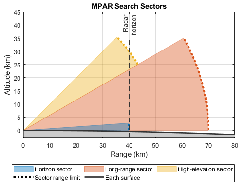
Set the horizon sector limits to -45 to 45 degrees in azimuth and 0 to 4 degrees in elevation, the long-range sector limits to -30 to 30 degrees in azimuth and 0 to 30 degrees in elevation, and the high-elevation sector limits to -45 to 45 degrees in azimuth and to 30 to 45 degrees in elevation.
% Number of search sectors
M = 3;

% Sector names
sectorNames = {'Horizon', 'Long-range', 'High-elevation'};

% Azimuth limits of the search sectors (deg)
azimuthLimits = [-45 -30 -45; 45 30 45];

% Elevation limits of the search sectors (deg)
elevationLimits = [0 0 30; 4 30 45];
The range limit of the horizon sector is determined by the distance beyond which a target becomes hidden by the horizon. Given the height of the radar platform this distance can be computed using the horizonrange function. The range limit of the long-range sector is determined by the instrumented range of the radar - the range beyond which the detection probability approaches zero. Finally, the range limit of the high-elevation sector is determined by the maximum target altitude. Set the range limits of the horizon, the long-range, and the high-elevation sectors to 40 km, 70 km, and 50 km respectively.
% Range limits (m)
rangeLimits = [40e3 70e3 50e3];
This example assumes that the MPAR performs surveillance of all three search sectors simultaneously. Since each sector has a different search volume, the search frame time,, is different for each sector. Additionally, each sector can have a different number of beam positions, . Assuming the dwell time, , (the time the beam spends in each beam position) is constant within a search sector, it is related to the search frame time as . Set the search frame time for the horizon sector to 0.5 seconds, for the long-range sector to 6 seconds, and for the high-elevation sector to 2 seconds.
% Search frame time
frameTime = [0.5 6 2];
The search frame times are selected such that the closure range covered by an undetected target in one scan is significantly smaller than the target range. Consider a target with the radial velocity of 250 m/s that emerges at a sector's range limit. Compute the closure range for this target in each search sector.
frameTime*250
ans = 1×3

         125        1500         500
In one scan this target will get closer to the radar by 125 m if it is in the horizon sector. Since the horizon sector covers targets that can emerge very close to the radar site, it is important that this sector is searched frequently and that an undetected target does not get too close to the radar before the next attempted detection. On the other hand, the range limit of the long-range sector is 70 km and the corresponding target closure distance is 1.5 km. Hence, an undetected target in the long-range sector will be able to cover only a small fraction of the sector's range limit in a single scan.
For convenience, organize the search sector parameters into an array of structs.
searchSectorParams(M) = helperSearchSector();

for i = 1:M
    searchSectorParams(i).SectorName = sectorNames{i};
    searchSectorParams(i).AzimuthLimits = azimuthLimits(:, i);
    searchSectorParams(i).ElevationLimits = elevationLimits(:, i);
    searchSectorParams(i).RangeLimit = rangeLimits(i);
    searchSectorParams(i).FrameTime = frameTime(i);
end
Quality-of-Service Resource Management
Under normal operational conditions the surveillance function is typically allocated enough resources such that the required detection performance is achieved in each search sector. But in circumstances when the surveillance function must compete for the radar resources with other radar functions, the RRM might allocate only a fraction of the desired resources to each search sector. These resources can be allocated based on hard rules such as sector priorities. However, coming up with rules that provide optimal resource allocation under all operational conditions is very difficult. A more flexible approach is to assign a metric to each task to describe the quality of the performed function [3]. The performance requirements can be specified in terms of the task quality, and the RRM can adjust the task control parameters to achieve these requirements.
This example assumes that resources are allocated to the search sectors in a form of PAP while the sectors' search frame times remain constant. It is convenient to treat PAP as a resource because it captures both the power and the aperture budget of the system. The presented resource allocation approach can be further extended to also include the search frame time to optimize the time budget of the system.
Let be a quality metric that describes performance of a search task created for the th sector. Here is the power aperture allocated by the RRM to the th sector, and is the set of control and environmental parameters for the th sector. To allocate the optimal amount of PAP to each search sector, the radar resource manager must solve the following optimization problem
such that
where
is the total number of search sectors;
is a vector that specifies the PAP allocation to each search sector;
is the total amount of PAP available to the MPAR's surveillance function;
is the utility function for th search sector;
and is the weight describing the priority of the th search sector.
Prior to weighting each sector with a priority weight, the QoS optimization problem first maps the quality of the th search tasks to the utility space. Such mapping is necessary because different tasks can have very different desired quality levels or even use entirely different metrics to express the task quality. A utility function associates a degree of satisfaction with each quality level according to the mission objectives. Optimizing the sum of weighted utilities across all tasks aims to allocate resources such that the overall satisfaction with the surveillance function is maximized.
Search Task Quality
The goal of a search task is to detect a target. As a target enters a search sector, it can be detected by the radar over multiple scans. With each scan the cumulative probability of detection grows as the target approaches the radar site. Therefore, a convenient metric that describes quality of a search task is the cumulative detection range - the range at which the cumulative probability of detection reaches a desired value of [4]. A commonly used is 0.9 and the corresponding cumulative detection range is denoted as .
Cumulative Probability of Detection
Let be the range limit of a search sector beyond which the probability of detecting a target can be assumed to be equal to zero. The cumulative detection probability for a target that entered the search sector at is then a function of the target range , the target radial speed , and the sector frame time
where
is the single-look probability of detection computed at range ;
is the number of completed scans until the target reaches the range from ;
is the closure range (distance traveled by the target in a single scan);
is the expectation taken with respect to the uniformly distributed random variable that represents the possibility of the target entering the search volume at any time within a scan.
Assuming a Swerling 1 case target and that all pulses within a dwell are coherently integrated, the single-look detection probability at range is
where is the probability of false alarm;
and is the reference SNR measured at the sector's range limit .
It follows from the radar search equation that depends on the PAP allocated to the search sector.
where
is the volume of the sector;
is the system temperature;
is the combined operational loss;
is the target radar cross section (RCS);
and is the Boltzmann's constant.
Use the solidangle function to compute the volume of a search sector and the radareqsearchsnr function to solve the radar search equation for . Then use the helperCumulativeDetectionProbability function to compute the cumulative detection probability as a function of the target range given the found .
First, assume that the system noise temperature is the same for each search sector and is equal to 913 K.
% System noise temperature (K)
Ts = [913 913 913];
Then, set the operational loss term for each sector.
% Operational loss (dB)
Loss = [22 19 24];
Accurate estimation of the operational loss term is critical to the use of the radar equation. It corrects for the assumption of an ideal system and an ideal environment. The operational loss includes contributions that account for environmental conditions, target positional uncertainty, scan loss, hardware degradation, and many other factors typically totaling dB or more [1, 2]. For more information on losses that must be included in the radar equation refer to Introduction to Introduction to Pulse Integration and Fluctuation Loss in Radar, Introduction to Scanning and Processing Losses in Pulse Radar, and Modeling the Propagation of Radar Signals examples.
Set the radial speed of the target to 250 m/s and the target RCS to 1 m². This example assumes that the radar is searching for the same kind of target in all three search sectors. In practice, the radial velocity and the RCS of a typical target of interest can be different for each search sector.
% Target radial speed (m/s)
[searchSectorParams.TargetRadialSpeed] = deal(250);

% Target RCS (m²)
[searchSectorParams.TargetRCS] = deal(1);
Finally, set the false alarm probability to 1e-6.
% Probability of false alarm
[searchSectorParams.FalseAlarmProbability] = deal(1e-6);
Consider different values of the PAP allocated to each sector.
% Allocated PAP (W*m^2)
pap = [20 40 80];
Compute the cumulative probability of detection.
% Target range
R = 20e3:0.5e3:80e3;

% Search sector volume (sr)
sectorVolume = zeros(M, 1);

figure
tiledlayout(3, 1, 'TileSpacing', 'tight')

for i = 1:M
    % Volume of the search sector
    sectorVolume(i) = solidangle(searchSectorParams(i).AzimuthLimits, searchSectorParams(i).ElevationLimits);

    % Store loss and system noise temperature in the sector parameters
    % struct
    searchSectorParams(i).OperationalLoss = Loss(i);
    searchSectorParams(i).SystemNoiseTemperature = Ts(i);

    % SNR at the sector's range limit
    SNRm = radareqsearchsnr(searchSectorParams(i).RangeLimit, pap, sectorVolume(i), searchSectorParams(i).FrameTime,...
        'RCS', searchSectorParams(i).TargetRCS, 'Ts', searchSectorParams(i).SystemNoiseTemperature, 'Loss', searchSectorParams(i).OperationalLoss);

    % Cumulative probability of detection
    Pc = helperCumulativeDetectionProbability(R, SNRm, searchSectorParams(i));

    % Plot
    ax = nexttile;
    colororder(flipud(ax.ColorOrder));

    hold on
    plot(R*1e-3, Pc, 'LineWidth', 2)
    xline(searchSectorParams(i).RangeLimit*1e-3, ':', 'LineWidth', 1.2, 'Color', 'k', 'Alpha', 1.0)
    yline(0.9, 'LineWidth', 1.2, 'Alpha', 1.0)

    ylabel('P_c')
    title(sprintf('%s Sector', searchSectorParams(i).SectorName))

    grid on

    xlim([20 80])
    ylim([-0.05 1.05])
end

xlabel('Target range (km)')
legendStr = {sprintf('PAP=%.0f (W·m²)', pap(1)), sprintf('PAP=%.0f (W·m²)', pap(2)), sprintf('PAP=%.0f (W·m²)', pap(3))};
legend([legendStr 'Range limit', 'P_c = 0.9'], 'Location', 'southoutside', 'Orientation', 'horizontal', 'NumColumns', 3)
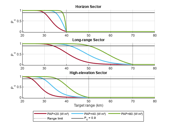
Beyond the sector's range limit a target is undetectable and the cumulative detection probability is zero. Starting at the sector's range limit, as the target approaches the radar, the number of detection attempts increases with each scan. Thus, the cumulative detection probability increases as the target range decreases. By varying the allocated PAP for each sector, the radar can vary the range.
Cumulative Detection Range
The range at which the cumulative detection probability equals 0.9, can be found by numerically solving equation with respect to the range variable .
Compute in each sector as the function of the allocated PAP.
% The desired cumulative detection probability in the sector
[searchSectorParams.CumulativeDetectionProbability] = deal(0.9);

% Power-aperture product (W·m²)
PAP = 1:2:600;

% Range at which the cumulative detection probability is equal to the
% desired value
R90 = zeros(M, numel(PAP));

str1 = cell(1, M);
str2 = cell(1, M);
for i = 1:M
    for j = 1:numel(PAP)
        % SNR at the sector's range limit
        SNRm = radareqsearchsnr(searchSectorParams(i).RangeLimit, PAP(j), sectorVolume(i), searchSectorParams(i).FrameTime,...
            'RCS', searchSectorParams(i).TargetRCS, 'Ts', searchSectorParams(i).SystemNoiseTemperature, 'Loss', searchSectorParams(i).OperationalLoss);

        % Cumulative detection probability at the range r
        % minus the required value of 0.9
        func = @(r)(helperCumulativeDetectionProbability(r, SNRm, searchSectorParams(i))- searchSectorParams(i).CumulativeDetectionProbability);

        % Solve for range
        options = optimset('TolX', 0.0001);
        R90(i, j) = fzero(func, [1e-3 1] * searchSectorParams(i).RangeLimit, options);
    end

    str1{i} = sprintf('R_{90} (%s)', searchSectorParams(i).SectorName);
    str2{i} = sprintf('Range limit (%s)', searchSectorParams(i).SectorName);
end

% Plot
figure
hold on
hl = plot(PAP, R90*1e-3, 'LineWidth', 2);
hy = yline([searchSectorParams.RangeLimit]*1e-3, ':', 'LineWidth', 1.5, 'Alpha', 1.0);
[hy.Color] = deal(hl.Color);

xlabel('Power-aperture product (W·m²)')
ylabel('R_{90} (km)')
ylim([0 80])

legend([str1 str2], 'Location', 'southeast')
title('Search Task Quality vs. Resource')
grid on
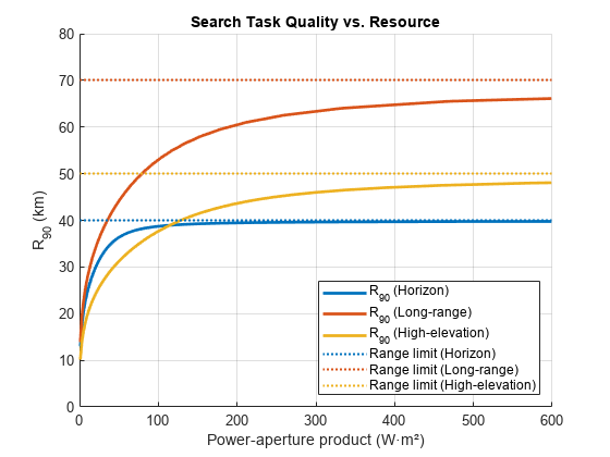
This result shows for each search sector the dependence of the search task quality,, on the allocated resource, the PAP. The RRM can allocate less or more PAP to a search sector to decrease or increase the effective value of . However, as the allocated PAP increases, approaches the asymptotic value bounded by the sector's range limit. If is already close to the sector's range limit, allocating more PAP to the sector will not provide any significant increase in the search task quality.
Search Task Utility
The QoS optimization problem seeks to find a resource allocation that jointly optimizes search quality across all sectors. Since the different values of can be desirable by different search sectors, simply maximizing the sum of the cumulative detection ranges will not result in a fair resource allocation. In that case search sectors with large will contribute significantly more to the objective function dominating search sectors with smaller . To account for differences in the desired values of across the sectors, the QoS optimization problem first maps the quality metric to a utility. The utility describes the degree of satisfaction with how the search task is performing. The joint utility can be maximized by first weighting and then summing the utilities of the individual tasks.
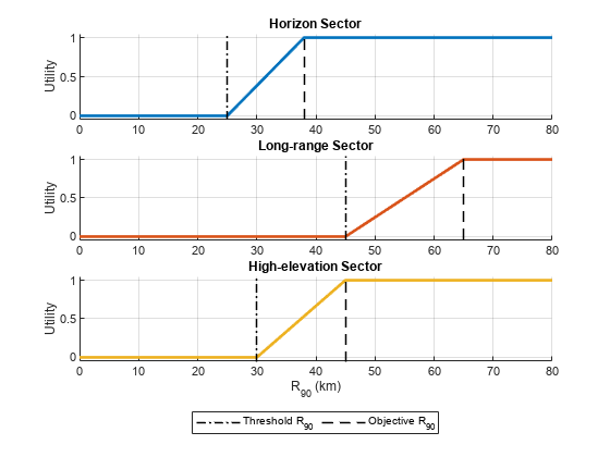
A simple utility function for a search task can be defined as follows [4]
where and are respectively the threshold and the objective value for in the sector . The objective determines the desired detection performance for a search sector, while the threshold is a value of the cumulative detection range below which the search task performance is considered unsatisfactory. The intuition behind this utility function is that if the task's quality is above the objective, allocating more resources to this task is wasteful since it will not increase the overall system's satisfaction with the search performance. Similarly, if the quality is below the threshold the utility is zero, and the RRM should allocate resources to the task only when it has enough resources to make the utility positive. The sector's utility is always between 0 and 1 regardless of the which makes it convenient to weight and add utilities across the sectors to obtain the joint utility for the surveillance function.
Define sets of objective and threshold values for each search sector.
% Objective range for each sector
Ro = [38e3 65e3 45e3];

% Threshold range for each sector
Rt = [25e3 45e3 30e3];
Create a utility function for each search sector using helperUtilityFunction and then plot it against the range.
% Ranges at which evaluate the utility functions
r90 = 0:1e3:80e3;

figure
tiledlayout(3, 1, 'TileSpacing', 'tight')
for i = 1:M
    % Store threshold and objective values for cumulative detection range
    % in the sector parameters struct
    searchSectorParams(i).ThresholdDetectionRange = Rt(i);
    searchSectorParams(i).ObjectiveDetectionRange = Ro(i);

    % Evaluate and plot the utility at different ranges
    ax = nexttile;
    colors = ax.ColorOrder;

    hold on
    plot(r90*1e-3, helperUtilityFunction(r90, Rt(i), Ro(i)), 'LineWidth', 2, 'Color', colors(i, :))
    ht = xline(Rt(i)*1e-3, '-.', 'Color', 'k', 'LineWidth', 1.2, 'Alpha', 1.0);
    ho = xline(Ro(i)*1e-3, '--', 'Color', 'k', 'LineWidth', 1.2, 'Alpha', 1.0);

    ylabel('Utility')
    ylim([-0.05 1.05])
    title(sprintf('%s Sector', searchSectorParams(i).SectorName))
    grid on
end
xlabel('R_{90} (km)')

legend([ht ho], {'Threshold R_{90}', 'Objective R_{90}'}, 'Location', 'southoutside', 'Orientation', 'horizontal')
Using these utility functions, the PAP (the resource) can be mapped to the utility.
figure
hold on
for i = 1:M
    plot(PAP, helperUtilityFunction(R90(i, :), Rt(i), Ro(i)), 'LineWidth', 2)
end

xlabel('Power-aperture product (W·m²)')
ylabel('Utility')
ylim([-0.05 1.05])
title('Utility vs. Resource')
grid on
legend({searchSectorParams.SectorName}, 'Location', 'best')
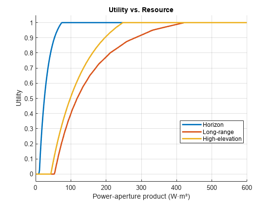
The long-range and the high-elevation sectors require about 50 W·m² of PAP to have a non-zero utility. At the same time, the utility of the horizon sector is maximized at 75 W·m² and allocating more PAP will not improve the objective of the QoS optimization problem. Overall, the horizon and the high-elevation sectors require less PAP than the long-range sector to achieve the same utility.
Utility Under Normal Operational Conditions
Assume that under the normal operational conditions the maximum utility is achieved in each search sector. In this case the RRM does not need to optimize the resource allocation. Each sector uses a nominal amount of resources enough to satisfy the corresponding objective requirement for the cumulative detection range.
Compute the PAP needed to achieve the maximum utility in each sector. First, find the SNR needed to achieve the cumulative probability of detection of 0.9 at the objective value of . Then use the radareqsearchpap function to solve the power-aperture form of the radar search equation to find the corresponding values of the PAP for the sectors.
% Power-aperture product
maxUtilityPAP = zeros(1, M);

for i = 1:M
    % Cumulative detection probability at the range Ro minus the required
    % value
    func = @(snr)(helperCumulativeDetectionProbability(Ro(i), snr, searchSectorParams(i)) ...
        - searchSectorParams(i).CumulativeDetectionProbability);

    % Solve for SNR
    options = optimset('TolX', 0.0001);
    snr = fzero(func, [-20 30], options);

    % PAP needed to make R90 equal to the objective range Ro
    maxUtilityPAP(i) = radareqsearchpap(searchSectorParams(i).RangeLimit, snr, sectorVolume(i), searchSectorParams(i).FrameTime,...
        'RCS', searchSectorParams(i).TargetRCS, 'Ts', searchSectorParams(i).SystemNoiseTemperature, 'Loss', searchSectorParams(i).OperationalLoss);
end

maxUtilityPAP
maxUtilityPAP = 1×3

   74.0962  421.6260  247.2633
The total amount of the PAP used by the surveillance function under the normal operation conditions is a sum of the maximum utility PAP values used by each sector.
% Total PAP needed for search under the normal operational conditions
normalSearchPAP = ceil(sum(maxUtilityPAP))
normalSearchPAP = 743
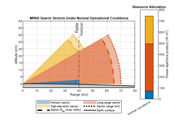
Use the provided helperDrawSearchSectors helper function to visualize the radar search sectors. This function also plots the objective value of for each sector - the cumulative detection range corresponding to the maximum utility. Use the bar chart to plot the PAP allocated to the sectors.
figure
tiledlayout(1, 6, 'TileSpacing', 'loose')

ax1 = nexttile([1 5]);
helperDrawSearchSectors(ax1, searchSectorParams, true);
title('MPAR Search Sectors Under Normal Operational Conditions')

nexttile
bar(categorical("Normal conditions"), maxUtilityPAP, 'stacked')
set(gca(), 'YAxisLocation', 'right')
ylabel('Power-aperture product (W·m²)')
title('Resource Allocation')
grid on
Solution to QoS Optimization Problem
Under the normal operational conditions all search tasks operate at the maximum utility, resulting in the cumulative detection range being equal or exceeding the objective value in each search sector. Since the total amount of resources available to MPAR is finite, activities of other radar functions such as tracking, maintenance, or communication, as well as system errors and failures can impose new constraints on the amount of resources accessible to the surveillance function. These deviations from the normal operational conditions prompt the RRM to recompute the resource allocations to the search tasks such that the new constraints are met, and the weighted utility is again maximized across all sectors.
The QoS optimization problem can be solved numerically using the fmincon function from the Optimization Toolbox™.
Set the sector priority weights such that the horizon sector has the highest priority, and the long-range sector has the lowest.
% Sector priority weights
w = [0.55 0.15 0.3];
Normalize the sector weights such that they add up to 1.
w = w/sum(w);
Assume that the surveillance function has access to only 50% of the PAP used for search under the normal operational conditions.
searchPAP = 0.5*normalSearchPAP
searchPAP =
371.5000
Set up the objective and the constraint functions.
% Objective function
fobj = @(x)helperQoSObjective(x, searchSectorParams, w);

% Constraint
fcon = @(x)helperQoSConstraint(x, searchPAP);
Set the lower and the upper bound on the QoS solution.
% Lower bound on the QoS solution
LB = 1e-6*ones(M, 1);

% Upper bound on the QoS solution
UB = maxUtilityPAP;
As the initial point for the optimization distribute the available PAP according to the sector priority weights.
% Starting points
startPAP = w*searchPAP;
Show the summary of the search sector parameters used to set up the QoS optimization problem.
helperSectorParams2Table(searchSectorParams)
ans=12×4 table
                Parameter                    Horizon          Long-range      High-elevation
    __________________________________    ______________    ______________    ______________

    {'AzimuthLimits'                 }    {2×1 double  }    {2×1 double  }    {2×1 double  }
    {'ElevationLimits'               }    {2×1 double  }    {2×1 double  }    {2×1 double  }
    {'RangeLimit'                    }    {[     40000]}    {[     70000]}    {[     50000]}
    {'FrameTime'                     }    {[    0.5000]}    {[         6]}    {[         2]}
    {'OperationalLoss'               }    {[        22]}    {[        19]}    {[        24]}
    {'SystemNoiseTemperature'        }    {[       913]}    {[       913]}    {[       913]}
    {'CumulativeDetectionProbability'}    {[    0.9000]}    {[    0.9000]}    {[    0.9000]}
    {'FalseAlarmProbability'         }    {[1.0000e-06]}    {[1.0000e-06]}    {[1.0000e-06]}
    {'TargetRCS'                     }    {[         1]}    {[         1]}    {[         1]}
    {'TargetRadialSpeed'             }    {[       250]}    {[       250]}    {[       250]}
    {'ThresholdDetectionRange'       }    {[     25000]}    {[     45000]}    {[     30000]}
    {'ObjectiveDetectionRange'       }    {[     38000]}    {[     65000]}    {[     45000]}
Use fmincon to find an optimal resource allocation.
options = optimoptions('fmincon', 'Display', 'off');
papAllocation = fmincon(fobj, startPAP, [], [], [], [], LB, UB, fcon, options)
papAllocation = 1×3

   74.0879  114.0092  183.4030
Verify that this allocation satisfies the constraint and does not exceed the available PAP amount.
sum(papAllocation)
ans =
371.5000
Given the found PAP allocations for each sector, compute and the corresponding value of the utility.
[~, optimalR90, utility] = helperQoSObjective(papAllocation, searchSectorParams, w)
optimalR90 = 1×3
104 ×

    3.8000    5.4581    4.3007
utility = 1×3

    1.0000    0.4791    0.8671
For the horizon sector, plot the found optimal resource allocation on the PAP vs. curve and the corresponding utility value on the utility vs. curve.
helperPlotR90AndUtility(PAP, R90(1, :), searchSectorParams(1), papAllocation(1), optimalR90(1), maxUtilityPAP(1), '#0072BD');
sgtitle({sprintf('%s Sector', searchSectorParams(1).SectorName), '(High Priority)'})
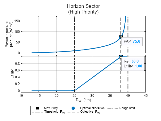
These plots visualize the two-step transformation performed inside the QoS optimization. The first step computes from the PAP, while the second step computes the utility from . To follow this transformation, start on the y-axis of the top subplot and choose a PAP value. Then find the corresponding point on the PAP vs. curve. Mark the value of this point on the x-axis. Using this value find a point on the utility curve in the bottom subplot. Finally, find the corresponding utility on the y-axis of the bottom subplot. The same set of steps can be traced in reverse to go from the utility to the PAP.
The surveillance function in this example is set up such that the horizon sector has the highest priority. It also requires much smaller PAP to achieve the objective compared to the other two sectors. The QoS optimization allocates 74.1 W·m² of PAP to the horizon sector. This is equal to the amount allocated to this sector under the normal operational conditions, resulting in the horizon sector utility approaching 1.
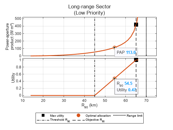
Plot the optimization results for the long-range and the high-elevation sectors.
helperPlotR90AndUtility(PAP, R90(2, :), searchSectorParams(2), papAllocation(2), optimalR90(2), maxUtilityPAP(2), '#D95319');
sgtitle({sprintf('%s Sector', searchSectorParams(2).SectorName), '(Low Priority)'})
helperPlotR90AndUtility(PAP, R90(3, :), searchSectorParams(3), papAllocation(3), optimalR90(3), maxUtilityPAP(3), '#EDB120');

sgtitle({sprintf('%s Sector', searchSectorParams(3).SectorName), '(Medium Priority)'})
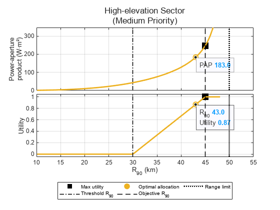
The QoS optimization allocates 114.2 W·m² and 183.25 W·m² to the long-range and the high-elevation sectors respectively. This allocation results in of about 55 km in the long-range sector, which corresponds to the utility of 0.5. The range in the high-elevation sector is equal to 43 km and the utility is about 0.87. The high-elevation sector is favored by the QoS optimization over the long-range sector because the corresponding sector priority weight is higher.
Use the provided helperDrawSearchSectors helper function to visualize the radar search sectors with the optimal value of obtained from the QoS optimization. Then use the bar chart to plot the computed optimal PAP allocation and compare it to the PAP allocation under the normal operational conditions.
figure
tiledlayout(1, 6, 'TileSpacing', 'compact')

ax1 = nexttile([1 5]);
helperDrawSearchSectors(ax1, searchSectorParams, false, optimalR90);
title('MPAR Search Sectors When 50% of PAP Is Available')

nexttile
ax2 = bar(categorical(["Normal conditions", "50% available"]), [maxUtilityPAP; papAllocation], 'stacked');
set(gca(), 'YAxisLocation', 'right')
ylabel('Power-aperture product (W·m²)')
title('Resource Allocation')
grid on

Conclusions
This example develops a resource management scheme for the surveillance function of an MPAR with multiple search sectors. The example starts by defining parameters of three search sectors: horizon, long-range, and high-elevation. It then introduces the QoS optimization problem as a resource allocation scheme. The cumulative detection range is used as a performance measure describing the quality of a search task and the utility functions based on the threshold and objective values are used to map the quality into the utility space. Finally, the example shows how to solve the QoS optimization problem numerically to obtain the optimal allocation of PAP to the search sectors.
References
James A. Scheer, William L. Melvin, Principles of Modern Radar: Radar Applications, Volume 3. United Kingdom: Institution of Engineering and Technology, 2013.
Barton, David Knox. Radar equations for modern radar. Artech House, 2013.
Charlish, Alexander, Folker Hoffmann, Christoph Degen, and Isabel Schlangen. “The Development From Adaptive to Cognitive Radar Resource Management.” IEEE Aerospace and Electronic Systems Magazine 35, no. 6 (June 1, 2020): 8–19.
Hoffmann, Folker, and Alexander Charlish. "A resource allocation model for the radar search function." In 2014 International Radar Conference, pp. 1-6. IEEE, 2014.
Supporting Functions
helperSearchSector
Creates a struct with placeholders for search sector parameters.
type('helperSearchSector.m')function searchSector = helperSearchSector()
searchSector = struct('SectorName', [], 'AzimuthLimits', [], 'ElevationLimits', [], 'RangeLimit', [], ...
'FrameTime', [], 'OperationalLoss', [], 'SystemNoiseTemperature', [], ...
'CumulativeDetectionProbability', [], 'FalseAlarmProbability', [], 'TargetRCS', [], ...
'TargetRadialSpeed', [], 'ThresholdDetectionRange', [], 'ObjectiveDetectionRange', []);
end
helperCumulativeDetectionProbability
Compute cumulative detection probability given range, SNR at the sector's range limit, and sector parameters.
type('helperCumulativeDetectionProbability.m')function Pc = helperCumulativeDetectionProbability(R, SNRm, searchSector)
% The expectation and the dependency of the number of scans N on the target
% range make the exact computation of the cumulative detection probability
% difficult. Instead, it could be conveniently approximated by linearly
% interpolating the lower bound expression
%
% P_c(R) >= 0, when R <= Rm && R > Rm - dR
% P_c(R) >= 1 - prod(1 - P_d(Rm - n*dR)), when R <= Rm - n*dR and n = 1:N
%
% computed at ranges Rm-k*dR, k=0,1,...
% Normalize range to the target popup range
R = R/searchSector.RangeLimit;
% Normalized target closure range
dR = searchSector.FrameTime*searchSector.TargetRadialSpeed/searchSector.RangeLimit;
Pfa = searchSector.FalseAlarmProbability;
SNRm = db2pow(SNRm(:).');
M = numel(SNRm);
Pc = zeros(numel(R), M);
idxs = R < 1;
r = R(idxs);
N = numel(r);
p = zeros(N, M);
for i = 1:N
range = (1:-dR:max(r(i)-dR, 0)).';
if dR > r(i) && range(end) ~= 0
range = [range; 0];
end
Pd = zeros(numel(range), M);
SNR = (range(2:end).^(-4))*SNRm;
Pd(2:end,:) = 1 - cumprod(1 - Pfa.^(1./(1+SNR)), 1);
p(i, :) = interp1(range, Pd, r(i));
end
Pc(idxs, :) = p;
end
helperUtilityFunction
Utility function.
type('helperUtilityFunction.m')function u = helperUtilityFunction(r, Rt, Ro) u = zeros(size(r)); idxo = r > Ro; u(idxo) = 1; idxt = r < Rt; u(idxt) = 0; idxs = ~idxo & ~idxt; u(idxs) = (r(idxs)-Rt)/(Ro-Rt); end
helperWeightedUtility
Function that returns weighted utility given PAP allocations, sectors weights, and sector parameters.
type('helperQoSObjective.m')function [val, R90, utility] = helperQoSObjective(papAllocation, searchSectorParams, weights)
val = 0;
M = numel(searchSectorParams);
R90 = zeros(1, M);
utility = zeros(1, M);
for i = 1:M
if papAllocation(i) > 0
sectorVolume = solidangle(searchSectorParams(i).AzimuthLimits, searchSectorParams(i).ElevationLimits);
snr = radareqsearchsnr(searchSectorParams(i).RangeLimit, papAllocation(i), sectorVolume, searchSectorParams(i).FrameTime, ...
'RCS', searchSectorParams(i).TargetRCS, 'Ts', searchSectorParams(i).SystemNoiseTemperature, 'Loss', searchSectorParams(i).OperationalLoss);
func = @(r)(helperCumulativeDetectionProbability(r, snr, searchSectorParams(i)) - searchSectorParams(i).CumulativeDetectionProbability);
options = optimset('TolX', 0.00001);
R90(i) = fzero(func, [1e-6 1] * searchSectorParams(i).RangeLimit, options);
utility(i) = helperUtilityFunction(R90(i), searchSectorParams(i).ThresholdDetectionRange, searchSectorParams(i).ObjectiveDetectionRange);
val = val - weights(i)*utility(i);
end
end
end
helperConstraintPAP
Function that defines the constraint on the PAP.
type('helperQoSConstraint.m')function [c, ceq] = helperQoSConstraint(pap, total) c = []; ceq = sum(pap) - total; end