オフライン処理のための、DCA1000EVM キャプチャ カードの使用による、TI mmWave レーダー ボードからの生 ADC データの記録

R2024b 以降

この例では、Radar Toolbox Support Package for Texas Instruments® mmWave Radar Sensors を使用して、Texas Instruments (TI) レーダーから生の ADC レーダー データ (IQ データ) をバイナリ ファイルに読み取って記録し、その記録されたデータを解析する方法を示します。

この例では、TI mmWave レーダーから記録された ADC データを使用して、レンジ応答とレンジ-ドップラー応答を評価および可視化します。

必要な製品

• MATLAB®

• Radar Toolbox Support Package for Texas Instruments mmWave Radar Sensors

サポート パッケージのインストールの詳細については、TI mmWave ハードウェアのサポートのインストールおよびハードウェア セットアップの実行を参照してください。

必要なハードウェア

• DCA1000EVM に接続して生の ADC データ (IQ データ) を読み取ることをサポートする、サポートされている TI mmWave レーダー評価モジュール (EVM) の 1 つ (サポートされているボードを参照)

• USB ケーブル (Type A-Micro B)

• 5V、3A 電源アダプター (AWR1642BOOST ボード、IWR1642BOOST ボード、または IWRL1642BOOST ボードを使用する場合は、電源アダプターが 2 つ必要)

• DCA1000EVM キャプチャ カード

• Samtec ケーブル

• イーサネット ケーブル

ハードウェア セットアップ

ADC データを MATLAB に読み取るには、TI mmWave レーダー センサーを使用する前にセット アップしなければなりません。ハードウェア セットアップ手順を (ハードウェア セットアップ画面で説明されているとおりに) 完了してセンサーをセット アップします。ハードウェア セットアップを起動するには、以下のコマンドを実行し、画面に表示される手順に従います。

mmWaveRadarSetup

ハードウェア セットアップ画面の起動方法については、TI mmWave ハードウェアのサポートのインストールおよびハードウェア セットアップの実行を参照してください。

mmWave レーダーと DCA1000 キャプチャ カードへの接続

ハードウェア セットアップ プロセスが正常に完了したら、ボード名を指定して TI レーダー ボードと DCA1000 に接続できます。この例では、IWR6843ISK EVM を使用します。別の EVM を使用している場合は、それに応じてボード名を変更してください。

dca = dca1000("IWR6843ISK");

ホスト コンピューターに TI Radar ボードを 1 つだけ接続している場合、MATLAB はシリアル ポートの詳細を自動的に検出します。複数のボードを接続している場合、または MATLAB によってシリアル ポートの詳細が自動的に入力されない場合は、ConfigPort 引数を指定します。以下に例を示します。

dca = dca1000("IWR6843ISK",ConfigPort = "COM3")

お使いのボードに対応する Config ポートを識別するには、Identifying Serial Ports for TI mmWave Radar Connectionを参照してください。

TI レーダーの構成

TI mmWave レーダー ボードを構成するには、シリアル ポートを使用してコマンドのシーケンスをボードに送信しなければなりません。シーケンスには、チャープ プロファイル、サンプル レートなどを指定するコマンドが含まれます。dca1000 オブジェクトの ConfigFile プロパティを使用して、コマンドのシーケンスをボードに送信します。詳細については、Configure Radar Using a Configuration (.cfg) File for Reading Raw ADC (IQ) Dataを参照してください。

この例では、サポート パッケージに付属する既定の構成を使用します。

ADC データの記録、および記録されたデータのレンジ応答とレンジ ドップラー応答の計算と可視化

このセクションは 2 つの部分に分かれています。

1. DCA1000EVM キャプチャ カードを使用して TI レーダー ボードから ADC データを記録します。

2. 記録されたファイルからレーダー データ キューブを読み取り、データのレンジ応答とレンジ ドップラー応答を計算して可視化します。

DCA1000EVM キャプチャ カードを使用して TI レーダー ボードから ADC データを記録します。

dca1000 オブジェクトのプロパティを使用して、記録パラメーター (記録時間、記録場所など) を設定できます。dca1000 オブジェクトの関数 startRecording を使用すると、TI レーダー ボードから ADC データを読み取り、指定された記録場所に他のメタデータとともにバイナリ形式で記録できます。

以下のスクリプトは、指定された recordLocation に TI レーダー ボードから 100 秒間の ADC データを読み取り、保存します。

メモ: startRecording 関数を使用して記録を開始すると、ポップアップ ウィンドウが表示されます。記録中はこのウィンドウを閉じないでください。記録が停止すると、ウィンドウは自動的に閉じます。

clear dca
% Create connection to the TI Radar board and DCA1000EVM Capture card
dca = dca1000("IWR6843ISK");
% Specify the duration to record ADC data
dca.RecordDuration = 100;
% Specify the location at which you want to store the recorded data along
% with the recording parameters
dca.RecordLocation = "C:\TIRadarADCData\dca1000Data";
% Start recording.
% The function startRecording opens a window. Ensure that you do not
% close this window. It will automatically close when the recording
% finishes.
startRecording(dca);
% The startRecording function captures data in background.
% While this is happening, you are free to utilize MATLAB for any other
% tasks you might need to perform. The following code is designed to
% prevent MATLAB from proceeding until the recording has finished.
% The isRecording() function will return true if the recording is still
% in progress. Once the recording has concluded or if it has not started,
% the function will return false.
while isRecording(dca)
end
% Remember the record location for post-processing.
% In this example, we will save the recording location in a variable.
recordLocation = dca.RecordLocation;
% Clear the dca1000 object and remove the hardware connections if required
clear dca

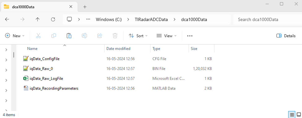
次のイメージは、ADC データ記録とともに生成されたファイルのサンプルを示しています。

記録時間を固定するのではなく、必要なだけ柔軟に記録するオプションがあります。これを有効にするには、dca1000 オブジェクトの RecordDuration プロパティを inf に設定します。記録を停止する準備ができたら、dca1000 オブジェクトの stopRecording 関数を使用します。

記録されたファイルからレーダー データ キューブを読み取り、データのレンジ応答とレンジ ドップラー応答を計算して可視化します。

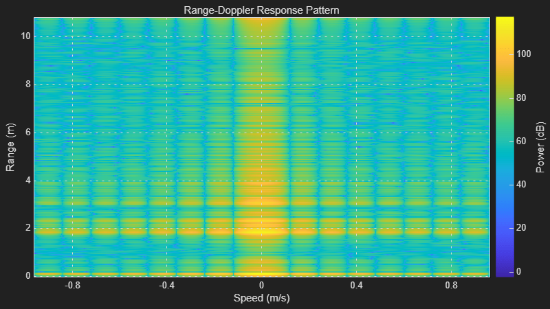
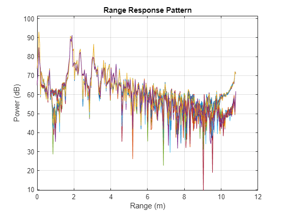
これらの記録されたバイナリ ファイルから ADC データ (IQ データ) キューブを読み取るには、dca1000FileReader System object を利用できます。phased.RangeResponse System object™ は、FFT ベースのアルゴリズムを使用して、ファストタイム (レンジ) データのレンジ フィルター処理を実行するために使用されます。phased.RangeResponse の plotResponse 関数は、入力データのレンジ応答をプロットするために使用されます。phased.RangeDopplerScope は、レンジ-ドップラー応答マップを計算して表示します。

% Load the recording parameters and Radar Configurations from the record
% location. This data is stored as a .mat file in the record location
temp = load(fullfile(recordLocation,'iqData_RecordingParameters.mat'));
dcaRecordingParams = temp.RecordingParameters;
% Define a variable to set the sampling rate in Hz for the
% phased.RangeResponse object. Because the dca1000 object provides the
% sampling rate in kHz, convert this rate to Hz.
fs = dcaRecordingParams.ADCSampleRate*1e3;
% Define a variable to set the FMCW sweep slope in Hz/s for the
% phased.RangeResponse object. Because the dca1000 object provides the
% sweep slope in GHz/us, convert this sweep slope to Hz/s.
sweepSlope = dcaRecordingParams.SweepSlope * 1e12;
% Define a variable to set the number of range samples
nr = dcaRecordingParams.SamplesPerChirp;
% Define a variable to set the center frequency in Hz for the
% phased.RangeDopplerScope object. Because the dca1000 object provides the
% center frequency in GHz, convert this rate to Hz.
fc = dcaRecordingParams.CenterFrequency*1e9;
% Define a variable to set the pulse repetition period in seconds for the
% phased.RangeDopplerScope object. Because the dca1000 object provides the
% chirp cycle time in us, convert this rate to seconds. The value is
% multiplied by 2 since in the example we are plotting the data only for first
% transmit channel out of 2 channels
tpulse = 2*dcaRecordingParams.ChirpCycleTime*1e-6;
% Pulse repetition interval
prf = 1/tpulse;
% Number of active receivers
nrx = dcaRecordingParams.NumReceivers;
% Number of chirps
nchirp = dcaRecordingParams.NumChirps;
% Create phased.RangeResponse System object that performs range filtering
% on fast-time (range) data, using an FFT-based algorithm
rangeresp = phased.RangeResponse(RangeMethod = 'FFT', ...
    RangeFFTLengthSource = 'Property', ...
    RangeFFTLength = nr, ...
    SampleRate = fs, ...
    SweepSlope = sweepSlope, ...
    ReferenceRangeCentered = false);
% Create range doppler scope to compute and display the response map.
rdscope = phased.RangeDopplerScope(IQDataInput=true, ...
    SweepSlope = sweepSlope,SampleRate = fs, ...
    DopplerOutput="Speed",OperatingFrequency=fc, ...
    PRFSource="Property",PRF=prf, ...
    RangeMethod="FFT",RangeFFTLength=nr, ...
    ReferenceRangeCentered = false);
% Create a dca1000FileReader object that enables you to read ADC data (IQ data) cubes
% from the binary files recorded using the object DCA1000 in MATLAB
fr = dca1000FileReader(recordLocation = recordLocation);
% Execute the loop till all the IQ data cubes are read from the record location
while (fr.CurrentPosition <= fr.NumDataCubes)
% Read a single IQ data cube from the binary file,
% starting from the location previously accessed.
iqData = read(fr,1);
% The function read() return cell array of IQ data cube,
% extract the radar data cube from it
iqData = iqData{1};
% Get the data from first receiver antenna
iqDataRx1 = squeeze(iqData(:,1,:));
% Plots the range response corresponding to the the input signal, iqData.
plotResponse(rangeresp, iqDataRx1);
% Get the data from first receiver antenna and first transmitter antenna
% (Every alternate pulse is from one transmitter antenna for this
% configuration)
iqDataRx1Tx1 = squeeze(iqData(:,1,1:2:end));
% Plots the range doppler response corresponding to the the input signal,
% iqData.
rdscope(iqDataRx1Tx1);
end