Estimate Range and Doppler Using Pulse Compression
This example shows the effects of pulse compression, where a transmitted pulse is modulated and correlated with the received signal. Radar and sonar systems use pulse compression to improve signal-to-noise ratio (SNR) and range resolution by shortening the duration of echoes. This example also demonstrates Doppler processing, where the radial velocity of a target is determined from the Doppler shift created by target motion.
Determining Range and Speed of Targets
The following radar system propagates a pulse train of linear frequency modulated (FM) waveforms to a moving target and receives the echoes. By applying matched filtering and Doppler processing to the echoes, the radar system can effectively detect the range and speed of the target.
Specify the requirements for the radar system. This example uses a carrier frequency fc of 3 gHz and a sampling rate fs of 1 mHz.
fc = 3e9;
fs = 1e6;
c = physconst('LightSpeed');
Create the system objects to model a radar system. The system is monostatic. The transmitter is located at (0,0,0) and is stationary, while the target is located at (5000,5000,0) with a velocity of (25,25,0) with a radar cross-section (RCS) of 1 square meter.
antenna = phased.IsotropicAntennaElement('FrequencyRange',[1e8 10e9]);
transmitter = phased.Transmitter('Gain',20,'InUseOutputPort',true);
txloc = [0;0;0];
tgtloc = [5000;5000;0]; % Radial Dist ~= 7071 m
tgtvel = [25;25;0]; % Radial Speed ~= 35.4 m/s
target = phased.RadarTarget('Model','Nonfluctuating','MeanRCS',1,'OperatingFrequency',fc);
antennaplatform = phased.Platform('InitialPosition',txloc);
targetplatform = phased.Platform('InitialPosition',tgtloc,'Velocity',tgtvel);
radiator = phased.Radiator('PropagationSpeed',c,...
   'OperatingFrequency',fc,'Sensor',antenna);
channel = phased.FreeSpace('PropagationSpeed',c,...
   'OperatingFrequency',fc,'TwoWayPropagation',false);
collector = phased.Collector('PropagationSpeed',c,...
   'OperatingFrequency',fc,'Sensor',antenna);
receiver = phased.ReceiverPreamp('NoiseFigure',0,...
   'EnableInputPort',true,'SeedSource','Property','Seed',2e3);
Create a linear FM waveform with a pulse width of 10 μs, a pulse repetition frequency of 10 kHz, and a sweep bandwidth of 100 kHz. The matched filter coefficients are generated from this waveform.
waveform = phased.LinearFMWaveform('PulseWidth',10e-6,'PRF',10e3,'OutputFormat','Pulses','NumPulses',1,'SweepBandwidth',1e5);
wav = waveform();
c = physconst('LightSpeed');
maxrange = c/(2*waveform.PRF);
SNR = npwgnthresh(1e-6,1,'noncoherent');
lambda = c/fc;
tau = waveform.PulseWidth;
Ts = 290;

filter = phased.MatchedFilter(...
   'Coefficients',getMatchedFilter(waveform),...
   'GainOutputPort',true);
To improve the Doppler resolution, the system emits 64 pulses, and the echoes are stored in rxsig. The data matrix stores the fast time samples (time within each pulse) along each column and the slow time samples (time between pulses) along each row.
numPulses = 64;
rxsig = zeros(length(wav),numPulses);

for n = 1:numPulses
    [tgtloc,tgtvel] = targetplatform(1/waveform.PRF);
    [tgtrng,tgtang] = rangeangle(tgtloc,txloc);

    [txsig, txstatus] = transmitter(wav);
    txsig = radiator(txsig,tgtang);
    txsig = channel(txsig,txloc,tgtloc,[0;0;0],tgtvel);
    txsig = target(txsig);
    txsig = channel(txsig,tgtloc,txloc,tgtvel,[0;0;0]);
    txsig = collector(txsig,tgtang);
    rxsig(:,n) = receiver(txsig,~txstatus);
end

prf = waveform.PRF;
fs = waveform.SampleRate;
response = phased.RangeDopplerResponse('DopplerFFTLengthSource','Property','DopplerFFTLength',2048,'SampleRate',fs,'DopplerOutput','Speed','OperatingFrequency',fc,'PRFSource','Property','PRF',prf);
filt = getMatchedFilter(waveform);
[resp,rng_grid,dop_grid] = response(rxsig,filt);

plotResponse(response,rxsig,filt,'Unit','db')
ylim([0 12000])
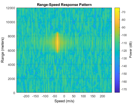
The response shows that the target is moving at about –40 m/s, and that the target is moving away from the transmitter since the speed is negative.
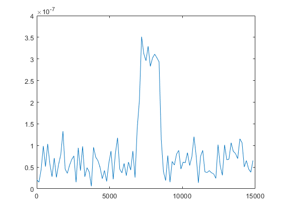
Calculate the range gates corresponding to the travel speed of the signal. The plot of the first slow time sample shows the largest peak around 7000 m, which corresponds with the range-speed response pattern plot.
fasttime = unigrid(0,1/fs,1/prf,'[)');
rangebins = (physconst('Lightspeed')*fasttime/2);

plot(rangebins,abs(rxsig(:,1)))
Determining Range
Create a threshold where the probability of false alarm is less than 1e-6. Use noncoherent integration of the 64 pulses assuming that the signal is in white Gaussian noise. Take the largest peak above the threshold and display the estimated target range.
pfa = 1e-6;
NoiseBandwidth = 5e6/2;
npower = noisepow(NoiseBandwidth, receiver.NoiseFigure,receiver.ReferenceTemperature);
thresh = npwgnthresh(pfa,numPulses,'noncoherent');
thresh = npower*db2pow(thresh);
[pks,range_detect] = findpeaks(pulsint(rxsig,'noncoherent'),'MinPeakHeight',thresh,'SortStr','descend');
range_estimate = rangebins(range_detect(1));
fprintf("Range Estimate: %3.2f m", range_estimate);
Range Estimate: 7344.92 m
Determining Speed
Take the slow-time samples corresponding to the range bin containing the detected target and plot the power spectral density estimate of the slow-time samples using the periodogram function.
ts = rxsig(range_detect(1),:).';
periodogram(ts,[],256,prf,'centered')
The peak frequency corresponds to the Doppler shift divided by 2, which can be converted into target speed. A positive speed means that the target is approaching the transmitter, while a negative speed indicates that the target is moving away from the transmitter.
[Pxx,F] = periodogram(ts,[],256,prf,'centered');

[Y,I] = max(Pxx);
lambda = physconst('Lightspeed')/fc;
tgtspeed = dop2speed(F(I)/2,lambda);
fprintf("Doppler Shift Estimate: %2.2f Hz",F(I)/2)
Doppler Shift Estimate: -351.56 Hz
fprintf("Speed Estimate: %2.2f m/s",tgtspeed)Speed Estimate: -35.13 m/s