Polarized Fields
Introduction to Polarization
You can use the Phased Array System Toolbox™ software to simulate radar systems that transmit, propagate, reflect, and receive polarized electromagnetic fields. By including this capability, the toolbox can realistically model the interaction of radar waves with targets and the environment.
It is a basic property of plane waves in free-space that the directions of the electric and magnetic field vectors are orthogonal to their direction of propagation. The direction of propagation of an electromagnetic wave is determined by the Poynting vector
In this equation, E represents the electric field and H represents the magnetic field. The quantity, S, represents the magnitude and direction of the wave’s energy flux. Maxwell’s equations, when applied to plane waves, produce the result that the electric and magnetic fields are related by
The vector s, the unit vector in the S direction, represents the direction of propagation of the wave. The quantity, Z, is the wave impedance and is a function of the electric permittivity and the magnetic permeability of medium in which the wave travels.
After manipulating the two equations, you can see that the electric and magnetic fields are orthogonal to the direction of propagation
This last result proves that there are really only two independent components of the electric field, labeled Ex and Ey. Similarly, the magnetic field can be expressed in terms of two independent components. Because of the orthogonality of the fields, the electric field can be represented in terms of two unit vectors orthogonal to the direction of propagation.
The unit vectors together with the unit vector in direction of propagation
form a right-handed orthonormal triad. Later, these vectors and the coordinates they define will be related to the coordinates of a specific radar system. Because the electric and magnetic fields are determined by each other, only the properties of the electric field need be consider.
For a radar system, the electric and magnetic field are actually spherical waves, rather than plane waves. However, in practice, these fields are usually measured in the far field region or radiation zone of the radar source and are approximately plane waves. In the far field, the waves are called quasi-plane waves. A point lies in the far field if its distance, R, from the source satisfies R ≫D2/λ where D is a typical dimension of the source, whether it is a single antenna or an array of antennas.
Polarization applies to purely sinusoidal signals. The most general expression for a sinusoidal plane-wave has the form
The quantities Ex0 and Ey0 are the real-valued, non-negative, amplitudes of the components of the electric field and ϕx and ϕy are field’s phases. This expression is the most general one used for a polarized wave. An electromagnetic wave is polarized if the ratio of the amplitudes of its components and phase difference between it components do not change with time. The definition of polarization can be broadened to include narrowband signals, for which the bandwidth is small compared to the center or carrier frequency of the signal. The amplitude ratio and phases difference vary slowly with time when compared to the period of the wave and may be thought of as constant over many oscillations.
You can usually suppress the spatial dependence of the field and write the electric field vector as
Linear and Circular Polarization
The preceding equation for a polarized plane wave shows that the tip of the two-dimensional electric field vector moves along a path which lies in a plane orthogonal to field’s direction of propagation. The shape of the path depends upon the magnitudes and phases of the components. For example, if ϕx = ϕy, you can remove the time dependence and write
This equation represents a straight line through the origin with positive slope. Conversely, suppose ϕx = ϕy + π. Then, the tip of the electric field vector follows a straight line through the origin with negative slope
These two polarization cases are named linear polarized because the field always oscillates along a straight line in the orthogonal plane. If Ex0= 0, the field is vertically polarized, and if Ey0 = 0 the field is horizontally polarized.
A different case occurs when the amplitudes are the same, Ex = Ey, but the phases differ by ±π/2
By squaring both sides, you can show that the tip of the electric field vector obeys the equation of a circle
While this equation gives the path the vector takes, it does not tell you in what direction the electric field vector travels around the circle. Does it rotate clockwise or counterclockwise? The rotation direction depends upon the sign of π/2 in the phase. You can see this dependency by examining the motion of the tip of the vector field. Assume the common phase angle, ϕ = 0. This assumption is permissible because the common phase only determines starting position of the vector and does not change the shape of its path. First, look at the +π/2 case for a wave travelling along the s-direction (out of the page). At t=0, the vector points along the x-axis. One quarter period later, the vector points along the negative y-axis. After another quarter period, it points along the negative x-axis.
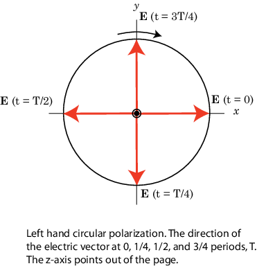
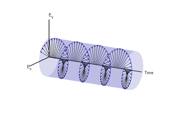
MATLAB® uses the IEEE convention to assign the names right-handed or left-handed polarization to the direction of rotation of the electric vector, rather than clockwise or counterclockwise. When using this convention, left or right handedness is determined by pointing your left or right thumb along the direction of propagation of the wave. Then, align the curve of your fingers to the direction of rotation of the field at a given point in space. If the rotation follows the curve of your left hand, then the wave is left-handed polarized. If the rotation follows the curve of your right hand, then the wave is right-handed polarized. In the preceding scenario, the field is left-handed circularly polarized (LHCP). The phase difference –π/2 corresponds to right-handed circularly polarized wave (RHCP). The following figure provides a three-dimensional view of what a LHCP electromagnetic wave looks like as it moves in the s-direction.
When the terms clockwise or counterclockwise are used they depend upon how you look at the wave. If you look along the direction of propagation, then the clockwise direction corresponds to right-handed polarization and counterclockwise corresponds to left-handed polarization. If you look toward where the wave is coming from, then clockwise corresponds to left-handed polarization and counterclockwise corresponds to right-handed polarization.
Left-Handed Circular Polarization
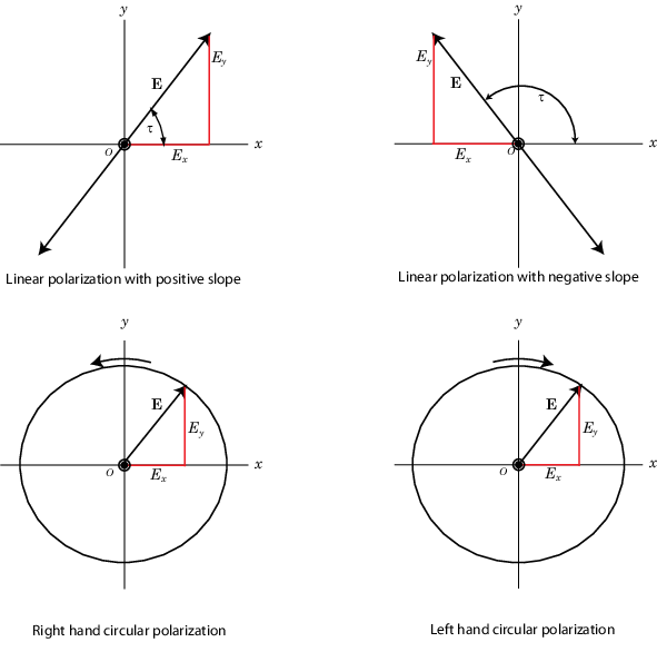
The figure below shows the appearance of linear and circularly polarized fields as they move towards you along the s-direction.
Linear and Circular Polarization
Elliptic Polarization
Besides the linear and circular states of polarization, a third type of polarization is elliptic polarization. Elliptic polarization includes linear and circular polarization as special cases.
As with linear or circular polarization, you can remove the time dependence to obtain the locus of points that the tip of the electric field vector travels
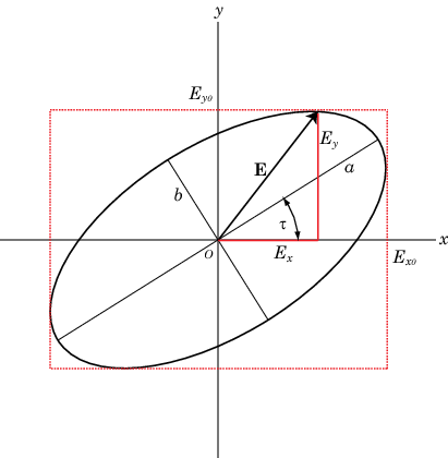
In this case, φ = φy – φx. This equation represents a tilted two-dimensional ellipse. Its size and shape are determined by the component amplitudes and phase difference. The presence of the cross term indicates that the ellipse is tilted. The equation does not, just as in the circularly polarized case, provide any information about the rotation direction. For example, the following figure shows the instantaneous state of the electric field but does not indicate the direction in which the field is rotating.
The size and shape of a two-dimensional ellipse can be defined by three parameters. These parameters are the lengths of its two axes, the semi-major axis, a, and semi-minor axis, b, and a tilt angle, τ. The following figure illustrates the three parameters of a tilted ellipse. You can derive them from the two electric field amplitudes and phase difference.
Polarization Ellipse
Polarization can best be understood in terms of complex signals. The complex representation of a polarized wave has the form
Define the complex polarization ratio as the ratio of the complex amplitudes
where ϕ = ϕy – ϕx.
It is useful to introduce the polarization vector. For the complex polarized electric field above, the polarization vector, P, is obtained by normalizing the electric field
where Em2 = Ex02 + Ey02 is the magnitude of the wave.
The overall size of the polarization ellipse is not important because that can vary as the wave travels through space, especially through geometric attenuation. What is important is the shape of the ellipse. Thus, the significant ellipse parameters are the ratio of its axis dimensions, a/b, called the axial ratio, and the tilt angle, τ. Both of these quantities can be determined from the ratio of the component amplitudes and the phase difference, or, equivalently, from the polarization ratio. Another quantity, equivalent to the axial ratio, is the ellipticity angle, ε.
In Phased Array System Toolbox, use the polratio function to convert the
complex amplitudes fv=[Eh;Ev] to the polarization ratio.
p = polratio(fv)
EH corresponds to
EX and
EV corresponds to
EV.Tilt Angle
The tilt angle is defined as the positive (counterclockwise) rotation angle from the x-axis to the semi-major axis of the ellipse. Because of the symmetry properties of the ellipse, the tilt angle, τ, need only be defined in the range –π/2 ≤ τ ≤ π/2. You can find the tilt angle by determining the rotated coordinate system in which the semi-major and semi-minor axes align with the rotated coordinate axes. Then, the ellipse equation has no cross-terms. The solution takes the form
where φ = φV – φH. Notice that you can rewrite this equation strictly in terms of the amplitude ratio and the phase difference.
Axial Ratio and Ellipticity Angle
After solving for the tilt angle, you can determine the semi-major and semi-minor axis lengths. Conceptually, you rotate the ellipse clockwise by the tilt angle and measure the lengths of the intersections of the ellipse with the H- and V-axes. The point of intersection with the larger value is the semi-major axis, a, and the one with the smaller value is the semi-minor axis, b.
The axial ratio is defined as AR = a/b and, by construction, is always greater than or equal to one. The ellipticity angle is defined by
and always lies in the range –π/4 ≤ ε ≤ π/4.
If you define the auxiliary angle, α, by
then, the ellipticity angle is given by
Both the axial ratio and ellipticity angle are defined from the amplitude ratio and phase difference and are independent of the overall magnitude of the field.
Rotation Sense
For elliptic polarization, just as with circular polarization, you need another parameter to completely describe the ellipse. This parameter must provide the rotation sense or the direction that the tip of the electric (or magnetic vector) moves in time. The rate of change of the angle that the field vector makes with the x-axis is proportion to –sin φ where φ is the phase difference. If sin φ is positive, the rate of change is negative, indicating that the field has left-handed polarization. If sin φ is negative, the rate of change is positive or right-handed polarization.
The function polellip lets you find the values
of the parameters of the polarization ellipse from either the field component
vector fv=[Eh;Ev] or the polarization ratio,
p.
fv=[Ey;Ex];
[tau,epsilon,ar,rs] = polellip(fv);
p = polratio(fv);
[tau,epsilon,ar,rs] = polellip(p);
tau, epsilon,
ar and rs represent the tilt angle,
ellipticity angle, axial ratio and rotation sense, respectively. Both syntaxes
give the same result.Polarization Value Summary
This table summaries several different common polarization states and the values of the amplitudes, phases, and polarization ratio that produce them:
| Polarization | Amplitudes | Phases | Polarization Ratio |
|---|---|---|---|
| Linear positive slope | Any non-negative real values for EH, EV. | φV = φH | Any non-negative real number |
| Linear negative slope | Any non-negative real values for EH, EV | φV = φH+ π | Any negative real number |
| Right-Handed Circular | EH=EV | φV= φH– π/2 | –i |
| Left-Handed Circular | EH=EV | φV= φH + π/2 | i |
| Right-Handed Elliptical | Any non-negative real values for EH, EV | sin (φV– φH) < 0 | sin(arg ρ) < 0 |
| Left-Handed Elliptical | Any non-negative real values for EH, EV | sin (φV– φH) >0 | sin(arg ρ) > 0 |
Linear and Circular Polarization Bases
As shown earlier, you can express a polarized electric field as a linear combination of basis vectors along the H and V directions. For example, the complex electric field vectors for the right-handed circularly polarized (RHCP) wave and the left-handed circularly polarized (LHCP) wave, take the form:
In this equation, the positive sign is for the LHCP field and the negative sign is for the RHCP field. These two special combinations can be given a new name. Define a new basis vector set, called the circular basis set
You can express any polarized field in terms of the circular basis set instead of the linear basis set. Conversely, you can also write the linear polarization basis in terms of the circular polarization basis
Any general elliptic field can be written as a combination of circular basis vectors
Jones Vector
The polarized field is orthogonal to the wave’s direction of propagation. Thus, the field can be completely specified by the two complex components of the electric field vector in the plane of polarization. The formulation of a polarized wave in terms of two-component vectors is called the Jones vector formulation. The Jones vector formulation can be expressed in either a linear basis or a circular basis or any basis. This table shows the representation of common polarizations in a linear basis and circular basis.
| Common Polarizations | Jones Vector in Linear Basis | Jones Vector in Circular Basis |
|---|---|---|
| Vertical | [0;1] | 1/sqrt(2)*[-1;1] |
| Horizontal | [1;0] | 1/sqrt(2)*[1;1] |
| 45° Linear | 1/sqrt(2)*[1;1] | 1/sqrt(2)*[1-1i;1+1i] |
| 135° Linear | 1/sqrt(2)*[1;-1] | 1/sqrt(2)*[1+1i;1-1i] |
| Right Circular | 1/sqrt(2)*[1;-1i] | [0;1] |
| Left Circular | 1/sqrt(2)*[1;1i] | [1;0] |
Stokes Parameters and the Poincaré Sphere
The polarization ellipse is an instantaneous representation of a polarized wave. However, its parameters, the tilt angle and the ellipticity angle, are often not directly measurable, particularly at very high frequencies such as light frequencies. However, you can determine the polarization from measurable intensities of the polarized field.
The measurable intensities are the Stokes parameters, S0, S1, S2, and S3. The first Stokes parameter, S0, describes the total intensity of the field. The second parameter, S1, describes the preponderance of linear horizontally polarized intensity over linear vertically polarized intensity. The third parameter, S2, describes the preponderance of linearly +45° polarized intensity over linearly 135° polarized intensity. Finally, S3 describes the preponderance of right circularly polarized intensity over left circularly polarized intensity. The Stokes parameters are defined as
For completely polarized fields, you can show by time averaging the polarization ellipse equation that
Thus, there are only three independent Stokes’ parameters.
For partially polarized fields, in contrast, the Stokes parameters satisfy the inequality
The Stokes parameters are related to the tilt and ellipticity angles, τ and ε
and inversely by
After you measure the Stokes’ parameters, the shape of the ellipse is completely determined by the preceding equations.
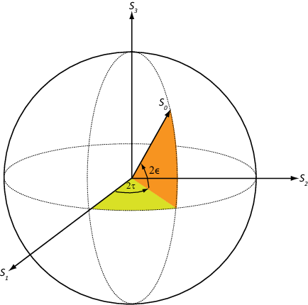
The two-dimensional Poincaré sphere can help you visualize the state of a polarized wave. Any point on or in the sphere represents a state of polarization determined by the four Stokes parameters, S0, S1, S2, and S3. On the Poincaré sphere, the angle from the S1-S2 plane to a point on the sphere is twice the ellipticity angle, ε. The angle from the S1- axis to the projection of the point into the S1-S2 plane is twice the tilt angle, τ.
As an example, solve for the Stokes parameters of a RHCP field,
fv=[1,-i], using the stokes function.
S = stokes(fv)
S =

     2
     0
     0
    -2
Sources of Polarized Fields
Antennas couple propagating electromagnetic radiation to electrical currents in wires, electromagnetic fields in waveguides or aperture fields. This coupling is a phenomenon common to both transmitting and receiving antennas. For some transmitting antennas, source currents in a wire produce electromagnetic waves that carrying power in all directions. Sometimes an antenna provides a means for a guided electromagnetic wave on a transmission line to transition to free-space waves such as a waveguide feeding a dish antennas. For receiving antennas, electromagnetic fields can induce currents in wires to generate signals to be then amplified and passed on to a detector.
For transmitting antennas, the shape of the antenna is chosen to enhance the power projected into a given direction. For receiving antennas, you choose the shape of the antenna to enhance the power received from a particular direction. Often, many transmitting antennas or receiving antennas are formed into an array. Arrays increase the transmitted power for a transmitting system or the sensitivity for a receiving system. They improve directivity over a single antenna.
An antenna can be assigned a polarization. The polarization of a transmitting antenna is the polarization of its radiated wave in the far field. The polarization of a receiving antenna is actually the polarization of a plane wave, from a given direction, resulting in maximum power at the antenna terminals. By the reciprocity theorem, all transmitting antennas can serve as receiving antennas and vice versa.
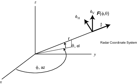
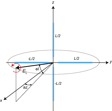
Each antenna or array has an associated local Cartesian coordinate system (x,y,z) as shown in the following figure. See Global and Local Coordinate Systems for more information. The local coordinate system can also be represented by a spherical coordinate system using azimuth, elevation and range coordinates, az, el, r, or alternately written, (φ,θ,r), as shown. At each point in the far field, you can create a set of unit spherical basis vectors, . The basis vectors are aligned with the (φ,θ,r) directions, respectively. In the far field, the electric field is orthogonal to the unit vector . The components of a polarized field with respect to this basis, (EH,EV), are called the horizontal and vertical components of the polarized field. In radar, it is common to use (H,V) instead of (x,y) to denote the components of a polarized field. In the far field, the polarized electric field takes the form
In this equation, the quantity F(φ,θ) is called the vector radiation pattern of the source and contains the angular dependence of the field in the far-field region.
Short Dipole Antenna Element
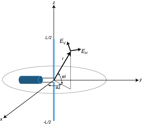
The simplest polarized antenna is the dipole antenna which consist of a split length of wire coupled at the middle to a coaxial cable. The simplest dipole, from a mathematical perspective, is the Hertzian dipole, in which the length of wire is much shorter than a wavelength. A diagram of the short dipole antenna of length L appears in the next figure. This antenna is fed by a coaxial feed which splits into two equal length wires of length L/2. The current, I, moves along the z-axis and is assumed to be the same at all points in the wire.
The electric field in the far field has the form
The next example computes the vertical and horizontal polarization components of the field. The vertical component is a function of elevation angle and is axially symmetric. The horizontal component vanishes everywhere.
The toolbox lets you model a short dipole antenna using the phased.ShortDipoleAntennaElement
System object™.
Short-Dipole Polarization Components
Compute the vertical and horizontal polarization components of the field created by a short-dipole antenna pointed along the z-direction. Plot the components as a function of elevation angle from 0° to 360°.
Create the phased.ShortDipoleAntennaElement System object™.
antenna = phased.ShortDipoleAntennaElement(...
    'FrequencyRange',[1,2]*1e9,'AxisDirection','Z');
Compute the antenna response. Because the elevation angle argument to antenna is restricted to ±90°, compute the responses for 0° azimuth and then for 180° azimuth. Combine the two responses in the plot. The operating frequency of the antenna is 1.5 GHz.
el = -90:90;
az = zeros(size(el));
fc = 1.5e9;
resp = antenna(fc,[az;el]);
az = 180.0*ones(size(el));
resp1 = antenna(fc,[az;el]);
Overlay the responses in the same figure.
figure(1)
subplot(121)
polarplot(el*pi/180.0,abs(resp.V.'),'b')
hold on
polarplot((el+180)*pi/180.0,abs(resp1.V.'),'b')
str = sprintf('%s\n%s','Vertical Polarization','vs Elevation Angle');
title(str)
hold off
subplot(122)
polarplot(el*pi/180.0,abs(resp.H.'),'b')
hold on
polarplot((el+180)*pi/180.0,abs(resp1.H.'),'b')
str = sprintf('%s\n%s','Horizontal Polarization','vs Elevation Angle');
title(str)
hold off
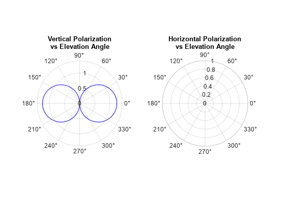
The plot shows that the horizontal component vanishes, as expected.
Crossed Dipole Antenna Element
You can use a cross-dipole antenna to generate circularly-polarized radiation. The crossed-dipole antenna consists of two identical but orthogonal short-dipole antennas that are phased 90° apart. A diagram of the crossed dipole antenna appears in the following figure. The electric field created by a crossed-dipole antenna constructed from a y-directed short dipole and a z-directed short dipole has the form
The polarization ratio EV/EH, when evaluated along the x-axis, is just –i which means that the polarization is exactly RHCP along the x-axis. It is predominantly RHCP when the observation point is close to the x-axis. Moving away from the x-axis, the field becomes a mixture of LHCP and RHCP polarizations. Along the –x-axis, the field is LHCP polarized. The figure illustrates, for a point near the x, that the field is primarily RHCP.
The toolbox lets you model a crossed-dipole antenna using the phased.CrossedDipoleAntennaElement
System object.
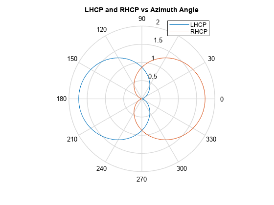
LHCP and RHCP Polarization Components
This example plots the right-hand and left-hand circular polarization components of fields generated by a crossed-dipole antenna at 1.5 GHz. You can see how the circular polarization changes from pure RHCP at 0 degrees azimuth angle to pure LHCP at 180 degrees azimuth angle, both at 0 degrees elevation angle.
Create the phased.CrossedDipoleAntennaElement object.
fc = 1.5e9;
antenna = phased.CrossedDipoleAntennaElement('FrequencyRange',[1,2]*1e9);
Compute the left-handed and right-handed circular polarization components from the antenna response.
az = [-180:180];
el = zeros(size(az));
resp = antenna(fc,[az;el]);
cfv = pol2circpol([resp.H.';resp.V.']);
clhp = cfv(1,:);
crhp = cfv(2,:);
Plot both circular polarization components at 0 degrees elevation.
polar(az*pi/180.0,abs(clhp))
hold on
polar(az*pi/180.0,abs(crhp))
title('LHCP and RHCP vs Azimuth Angle')
legend('LHCP','RHCP')
hold off
Arrays Supporting Polarization
You can create polarized fields from arrays by using polarized antenna
elements as a value of the Elements property of an array
System object. All Phased Array System Toolbox arrays support polarization.
Scattering Cross-Section Matrix
After a polarized field is created by an antenna system, the field radiates to the far-field region. When the field propagates into free space, the polarization properties remain unchanged until the field interacts with a material substance which scatters the field into many directions. In such situations, the amplitude and polarization of the scattered wave can differ from the incident wave polarization. The scattered wave polarization may depend upon the direction in which the scattered wave is observed. The exact way that the polarization changes depends upon the properties of the scattering object. The quantity describing the response of an object to the incident field is called the radar scattering cross-section matrix (RSCM), S. You can measure the scattering matrix as follows. When a unit amplitude horizontally polarized wave is scattered, both a horizontal and a vertical scattered component are produced. Call these two components SHH and SVH. These components are complex numbers containing the amplitude and phase changes from the incident wave. Similarly, when a unit amplitude vertically polarized wave is scattered, the horizontal and vertical scattered component produced are SHV and SVV. Because, any incident field can be decomposed into horizontal and vertical components, you can arrange these quantities into a matrix and write the scattered field in terms of the incident field
In general, the scattering cross-section matrix depends upon the angles that the incident and scattered fields make with the object. When the incident field is scattered back to the transmitting antenna or, backscattered, the scattering matrix is symmetric.
Polarization Signature
To understand how the scattered wave depends upon the polarization of the incident wave, you need to examine all possible scattered field polarizations for each incident polarization. Because this amount of data is difficult to visualize, consider two cases:
For the copolarization case, the scattered polarization has the same polarization as the incident field.
For the cross-polarization case, the scattered polarization has an orthogonal polarization to the incident field.
You can represent the incident polarizations in terms of the tilt angle-ellipticity angle pair . Every unit incident polarization vector can be expressed as
while the orthogonal polarization vector is
When you have an RSCM matrix, S, form the copolarization signature by computing
where []* denotes complex conjugation. To
obtain the cross-polarization signature, compute
You can compute both the copolarization and cross
polarization signatures using the polsignature function. This
function returns the absolute value of the scattered power (normalized by its
maximum value). The next example shows how to plot the polarization signatures
for the RSCM matrix
for all possible incident polarizations. The range of values of the ellipticity angle and tilt span the entire possible range of polarizations.
Plot Polarization Signatures
Plot the copolarization and cross-polarization signatures of the scattering matrix
Specify the scattering matrix. and specify the range of ellipticity angles and orientation (tilt) angles that define the polarization states. These angles cover all possible incident polarization states.
rscmat = [1i*2,0.5;0.5,-1i];
el = [-45:45];
tilt = [-90:90];
Plot the copolarization signatures for all incident polarizations.
polsignature(rscmat,'c',el,tilt)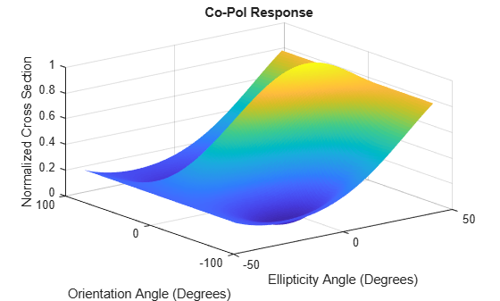
Plot the cross-polarizations signatures for all incident polarizations.
polsignature(rscmat,'x',el,tilt)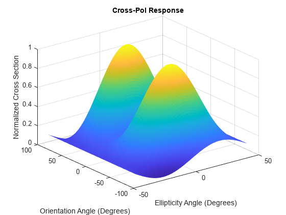
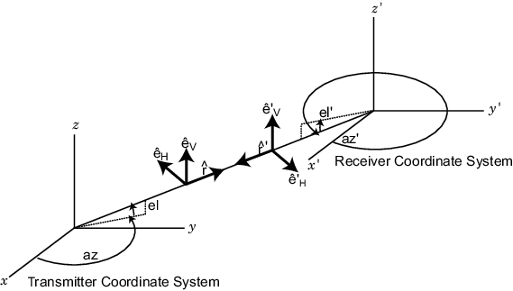
Polarization Loss Due to Field and Receiver Mismatch
An antenna that is used to receive polarized electromagnetic waves achieves its maximum output power when the antenna polarization is matched to the polarization of the incident electromagnetic field. Otherwise, there is polarization loss:
The polarization loss is computed from the projection (or dot product) of the transmitted field’s electric field vector onto the receiver polarization vector.
Loss occurs when there is a mismatch in direction of the two vectors, not in their magnitudes.
The polarization loss factor describes the fraction of incident power that has the correct polarization for reception.
Using the transmitter’s spherical basis at the receiver’s position, you can represent the incident electric field, (EiH, EiV), by
You can represent the receiver’s polarization vector, (PH, PV), in the receiver’s local spherical basis by:
The next figure shows the construction of the transmitter and receiver spherical basis vectors.
The polarization loss is defined by:
and varies between 0 and 1. Because the vectors are defined with
respect to different coordinate systems, they must be converted to the global
coordinate system to form the projection. The toolbox function polloss computes the polarization mismatch between an incident field
and a polarized antenna.
To achieve maximum output power from a receiving antenna, the matched antenna polarization vector must be the complex conjugate of the incoming field’s polarization vector. As an example, if the incoming field is RHCP, with polarization vector given by , the optimum receiver antenna polarization is LHCP. The introduction of the complex conjugate is needed because field polarizations are described with respect to its direction of propagation, whereas the polarization of a receive antenna is usually specified in terms of the direction of propagation towards the antenna. The complex conjugate corrects for the opposite sense of polarization when receiving.
As an example, if the transmitting antenna transmits an RHCP field, the polarization loss factors for various received antenna polarizations are
| Receive Antenna Polarization | Receive Antenna Polarization Vector | Polarization Loss Factor | Polarization Loss Factor (dB) |
|---|---|---|---|
| Horizontal linear | eH | 1/2 | 3 dB |
| Vertical linear | eV | 1/2 | 3 |
| RHCP | 0 | ∞ | |
| LHCP | 1 | 0 |
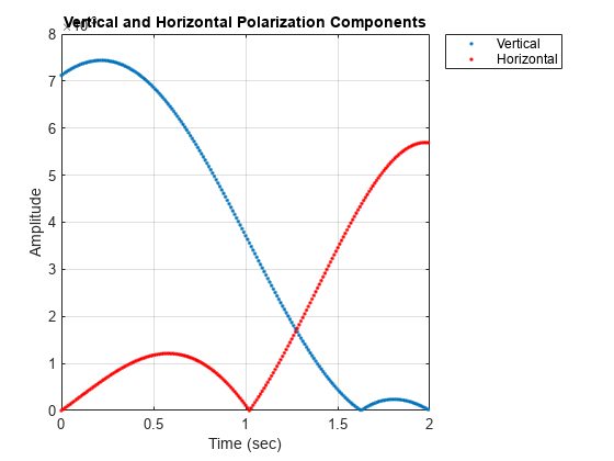
Model Radar Transmitting Polarized Radiation
This example models a tracking radar based on a 31-by-31 (961-element) uniform rectangular array (URA). The radar is designed to follow a moving target. At each time instant, the radar points in the known direction of the target. The basic radar requirements are the probability of detection, pd, the probability of false alarm, pfa, the maximum unambiguous range, max_range, and the range resolution, range_res, (all distance units are in meters). The range_gate parameter limits the region of interest to a range smaller than the maximum range. The operating frequency is set in fc. The simulation lasts for numpulses pulses.
Radar Definition
Set up the radar operating parameters. The existing radar design meets the following specifications.
pd = 0.9;            % Probability of detection
pfa = 1e-6;          % Probability of false alarm
max_range = 1500*1000; % Maximum unambiguous range
range_res = 50.0;    % Range resolution
rangegate = 5*1000;  % Assume all objects are in this range
numpulses = 200;     % Number of pulses to integrate
fc = 8e9;            % Center frequency of pulse
c = physconst('LightSpeed');
tmax = 2*rangegate/c; % Time of  echo from object at rangegate
Pulse Repetition Interval
Set the pulse repetition interval, PRI, and pulse repetition frequency, PRF, based on the maximum unambiguous range.
PRI = 2*max_range/c;
PRF = 1/PRI;
Transmitted Signal
Set up the transmitted rectangular waveform using the phased.RectangularWaveform System object™. The waveform pulse width, pulse_width, and pulse bandwidth, pulse_bw, are determined by the range resolution, range_res, that you select. Specify the sampling rate, fs, to be twice the pulse bandwidth. The sampling rate must be an integer multiple of the PRF. Therefore, modify the sampling rate to satisfy the requirement.
pulse_bw = c/(2*range_res);    % Pulse bandwidth
pulse_width = 1/pulse_bw;               % Pulse width
fs = 2*pulse_bw;                        % Sampling rate
n = ceil(fs/PRF);
fs = n*PRF;
waveform = phased.RectangularWaveform('PulseWidth',pulse_width,'PRF',PRF,...
    'SampleRate',fs);
Antennas and URA Array
The array consists of short-dipole antenna elements. Use the phased.ShortDipoleAntennaElement System object to create a short-dipole antenna oriented along the z-axis.
antenna = phased.ShortDipoleAntennaElement(...
    'FrequencyRange',[5e9,10e9],'AxisDirection','Z');
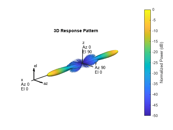
Define a 31-by-31 Taylor tapered uniform rectangular array using the phased.URA System object. Set the size of the array using the number of rows, numRows, and the number of columns, numCols. The distance between elements, d, is slightly smaller than one-half the wavelength, lambda. Compute the array taper, tw, using separate Taylor windows for the row and column directions. Obtain the Taylor weights using the taylorwin function. Plot the 3-D array response using the array pattern method.
numCols = 31;
numRows = 31;
lambda = c/fc;
d = 0.9*lambda/2; % Nominal spacing
wc = taylorwin(numCols);
wr = taylorwin(numRows);
tw = wr*wc';
array = phased.URA('Element',antenna,'Size',[numCols,numRows],...
    'ElementSpacing',[d,d],'Taper',tw);
pattern(array,fc,-180:180,-90:90,'CoordinateSystem','polar','Type','powerdb',...
    'Polarization','V');
Radar Platform Motion
Next, set the position and motion of the radar platform in the phased.Platform System object. The radar is assumed to be stationary and positioned at the origin. Set the Velocity property to [0,0,0] and the InitialPosition property to [0,0,0]. Set the InitialOrientationAxes property to the identity matrix to align the radar platform coordinate axes with the global coordinate system.
radarPlatformAxes = [1 0 0;0 1 0;0 0 1];
radarplatform = phased.Platform('InitialPosition',[0;0;0],...
    'Velocity',[0;0;0],'OrientationAxes',radarPlatformAxes);
Transmitters and Receivers
In radar, the signal propagates in the form of an electromagnetic wave. The signal is radiated and collected by the antennas used in the radar system. Associate the array with a radiator System object, phased.Radiator, and two collector System objects, phased.Collector. Set the WeightsInputPort property of the radiator to true to enable dynamic steering of the transmitted signal at each execution of the radiator. Creating the two collectors allows for collection of both horizontal and vertical polarization components.
radiator = phased.Radiator('Sensor',array,'OperatingFrequency',fc,...
    'PropagationSpeed',c,'CombineRadiatedSignals',true,...
    'Polarization','Combined','WeightsInputPort',true);
collector1 = phased.Collector('Sensor',array,'OperatingFrequency',fc,...
    'PropagationSpeed',c,'Wavefront','Plane','Polarization','Combined',...
    'WeightsInputPort',false);
collector2 = phased.Collector('Sensor',array,'OperatingFrequency',fc,...
    'PropagationSpeed',c,'Wavefront','Plane','Polarization','Combined',...
    'WeightsInputPort',false);
Estimate the peak power needed in the phased.Transmitter System object to calculate the desired radiated power levels. The transmitted peak power is the power required to achieve a minimum-detection SNR, snr_min. You can determine the minimum SNR from the probability of detection, pd, and the probability of false alarm, pfa, using the albersheim function. Then, compute the peak power, peak_power, from the radar equation. The peak power depends on the overall signal gain, which is the sum of the transmitting element gain, TransmitterGain and the array gain, AG. The peak power also depends on the maximum detection range, rangegate. Finally, you need to supply a target cross-section value, tgt_rcs. A scalar radar cross section is used in this code section as an approximation even though the full polarization computation later uses a 2-by-2 radar cross section scattering matrix.
Using the radar equation formula, estimate the total transmitted power to achieve a required detection SNR using all the pulses.
The SNR has contributions from the transmitting element gain as well as the array gain. Compute first an estimate of the array gain, then add the array gain to the transmitter gain to get the peak power which achieves the desired SNR.
Use an approximate target cross section of 1.0 for the radar equation even though the analysis calls for the full scattering matrix.
Set the maximum range to be equal to the value of 'rangegate' since targets outside that range are of no interest.
Compute the array gain as 10*log10(number of elements)
Assume each element has a gain of 20 dB.
snr_min = albersheim(pd, pfa, numpulses);
AG = 10*log10(numCols*numRows);
tgt_rcs = 1;
TransmitterGain = 20;
tau = waveform.PulseWidth;
Ts = 290;
dbterm = db2pow(snr_min - 2*TransmitterGain + AG);
peak_power = (4*pi)^3*physconst('Boltzmann')*Ts/tau/tgt_rcs/lambda^2*rangegate^4*dbterm
peak_power = 5.1778e+05
transmitter = phased.Transmitter('PeakPower',peak_power,'Gain',TransmitterGain,...
    'LossFactor',0,'InUseOutputPort',true,'CoherentOnTransmit',true);
Define Target
We want to simulate the pulse returns from a target that is rotating so that the scattering cross-section matrix changes from pulse to pulse. Create a rotating target object and a moving target platform. The rotating target is represented later as an angle-dependent scattering matrix. Rotation is in degrees per second.
targetSpeed = 1000;
targetVec = [-1;1;0]/sqrt(2);
target = phased.RadarTarget('EnablePolarization',true,...
    'Mode','Monostatic','ScatteringMatrixSource','Input port',...
    'OperatingFrequency',fc);
targetPlatformAxes = [1 0 0;0 1 0;0 0 1];
targetRotRate = 45;
targetplatform = phased.Platform('InitialPosition',[3500.0; 0; 0],...
    'Velocity', targetSpeed*targetVec);
Other System Objects
Steering vector defined by
phased.SteeringVectorSystem object.Beamformer defined by
phased.PhaseShiftBeamformerSystem object. TheDirectionSourceproperty is set to'Input Port'to enable the beamformer to always points towards the known target direction at each execution.Free-space propagator using the
phased.FreeSpaceSystem object.Receiver preamp model using the
phased.ReceiverPreampsystem object.
Signal Propagation
Because the reflected signals are received by an array, use a beamformer pointing to the steering direction to obtain the combined signal.
steeringvector = phased.SteeringVector('SensorArray',array,'PropagationSpeed',c,...
    'IncludeElementResponse',false);
beamformer = phased.PhaseShiftBeamformer('SensorArray',array,...
    'OperatingFrequency',fc,'PropagationSpeed',c,...
    'DirectionSource','Input port');
channel = phased.FreeSpace('SampleRate',fs,...
    'TwoWayPropagation',true,'OperatingFrequency',fc);
% Define a receiver with receiver noise
amplifier = phased.ReceiverPreamp('Gain',20,'LossFactor',0,'NoiseFigure',1,...
    'ReferenceTemperature',290,'SampleRate',fs,'EnableInputPort',true,...
    'PhaseNoiseInputPort',false,'SeedSource','Auto');
For such a large PRI and sampling rate, there will be too many samples per element. This will cause problems with the collector which has 961 channels. To keep the number of samples manageable, set a maximum range of 5 km. We know that the target is within this range.
This set of axes specifies the direction of the local coordinate axes with respect to the global coordinate system. This is the orientation of the target.
Processing Loop
Pre-allocate arrays for collecting data to be plotted.
sig_max_V  = zeros(1,numpulses);
sig_max_H  = zeros(1,numpulses);
tm_V = zeros(1,numpulses);
tm_H = zeros(1,numpulses);
After all the System objects are created, loop over the number of pulses to create the reflected signals.
maxsamp = ceil(tmax*fs);
fast_time_grid = (0:(maxsamp-1))/fs;
rotangle = 0.0;
for m = 1:numpulses
    x = waveform(); % Generate pulse
    % Capture only samples within range gated
    x = x(1:maxsamp);
    [s, tx_status] = transmitter(x);   % Create transmitted pulse
    % Move the radar platform and target platform.
    [radarPos,radarVel] = radarplatform(1/PRF);
    [targetPos,targetVel] = targetplatform(1/PRF);
    % Compute the known target angle
    [targetRng,targetAng] = rangeangle(targetPos,...
        radarPos,...
        radarPlatformAxes);
    % Compute the radar angle with respect to the target axes.
    [radarRng,radarAng] = rangeangle(radarPos,...
        targetPos,...
        targetPlatformAxes);
    % Calculate the steering vector designed to track the target
    sv = steeringvector(fc,targetAng);
    % Radiate the polarized signal toward the targat
    tsig1 = radiator(s,targetAng,radarPlatformAxes,conj(sv));
    % Compute the two-way propagation loss (4*pi*R/lambda)^2
    tsig2 = channel(tsig1,radarPos,targetPos,radarVel,targetVel);
    % Create a very simple model of a changing scattering matrix
    scatteringMatrix = [cosd(rotangle),0.5*sind(rotangle);...
        0.5*sind(rotangle),cosd(rotangle)];
    rsig1 = target(tsig2,radarAng,targetPlatformAxes,scatteringMatrix);  % Reflect off target
    % Collect the vertical component of the radiation.
    rsig3V = collector1(rsig1,targetAng,radarPlatformAxes);
    % Collect the horizontal component of the radiation. This
    % second collector is rotated around the x-axis to be more
    % sensitive to horizontal polarization
    rsig3H = collector2(rsig1,targetAng,rotx(90)*radarPlatformAxes);
    % Add receiver noise to both sets of signals
    rsig4V = amplifier(rsig3V,~(tx_status>0)); % Receive signal
    rsig4H = amplifier(rsig3H,~(tx_status>0)); % Receive signal
    % Beamform the signal
    rsigV = beamformer(rsig4V,targetAng); % Beamforming
    rsigH = beamformer(rsig4H,targetAng); % Beamforming
    % Find the maximum returns for each pulse and store them in
    % a vector. Store the pulse received time as well.
    [sigmaxV,imaxV] = max(abs(rsigV));
    [sigmaxH,imaxH] = max(abs(rsigH));
    sig_max_V(m) = sigmaxV;
    sig_max_H(m) = sigmaxH;
    tm_V(m) = fast_time_grid(imaxV) + (m-1)*PRI;
    tm_H(m) = fast_time_grid(imaxH) + (m-1)*PRI;

    % Update the orientation of the target platform axes
    targetPlatformAxes = ...
        rotx(PRI*targetRotRate)*targetPlatformAxes;
    rotangle = rotangle + PRI*targetRotRate;
end
% Plot the vertical and horizontal polarization for each pulse as a
% function of time.
plot(tm_V,sig_max_V,'.')
hold on
plot(tm_H,sig_max_H,'r.')
hold off
xlabel('Time (sec)')
ylabel('Amplitude')
title('Vertical and Horizontal Polarization Components')
legend('Vertical','Horizontal')
grid on