interpolateTemperature

Interpolate temperature in thermal result at arbitrary spatial locations

Syntax

Tintrp = interpolateTemperature(thermalresults,xq,yq)

Tintrp = interpolateTemperature(thermalresults,xq,yq,zq)

Tintrp = interpolateTemperature(thermalresults,querypoints)

Tintrp = interpolateTemperature(___,iT)

Description

Tintrp = interpolateTemperature(thermalresults,xq,yq) returns the interpolated temperature values at the 2-D points specified in xq and yq for a steady-state thermal model.

Tintrp = interpolateTemperature(thermalresults,xq,yq,zq) returns the interpolated temperature values at the 3-D points specified in xq, yq, and zq for a steady-state thermal model.

Tintrp = interpolateTemperature(thermalresults,querypoints) returns the interpolated temperature values at the points in querypoints for a steady-state thermal model.

Tintrp = interpolateTemperature(___,iT) returns the interpolated temperature values for the transient thermal model at times iT.

Examples

Interpolate Temperatures in 2-D Steady-State Thermal Problem

Create and plot a square geometry.

R1 = [3,4,-1,1,1,-1,1,1,-1,-1]';
g = decsg(R1, 'R1', ('R1')');
pdegplot(g,EdgeLabels="on")
xlim([-1.1,1.1])
ylim([-1.1,1.1])

Create an femodel object for steady-state thermal analysis and include the geometry into the model.

model = femodel(AnalysisType="thermalSteady", ...
                Geometry=g);

Assuming that this is an iron plate, assign a thermal conductivity of 79.5 W/(m*K). For steady-state analysis, you do not need to assign mass density or specific heat values.

model.MaterialProperties = ...
    materialProperties(ThermalConductivity=79.5);

Apply a constant temperature of 300 K to the bottom of the plate (edge 3).

model.EdgeBC(3) = edgeBC(Temperature=300);

Apply convection on the two sides of the plate (edges 2 and 4).

model.EdgeLoad([2 4]) = ...
    edgeLoad(ConvectionCoefficient=25,...
             AmbientTemperature=50);

Mesh the geometry and solve the problem.

model = generateMesh(model);
R = solve(model)

R = 
  SteadyStateThermalResults with properties:

    Temperature: [1529×1 double]
     XGradients: [1529×1 double]
     YGradients: [1529×1 double]
     ZGradients: []
           Mesh: [1×1 FEMesh]

The solver finds the values of temperatures and temperature gradients at the nodal locations. To access these values, use R.Temperature, R.XGradients, and so on. For example, plot the temperatures at nodal locations.

figure;
pdeplot(R.Mesh,XYData=R.Temperature,...
        Contour="on",ColorMap="hot");
axis equal

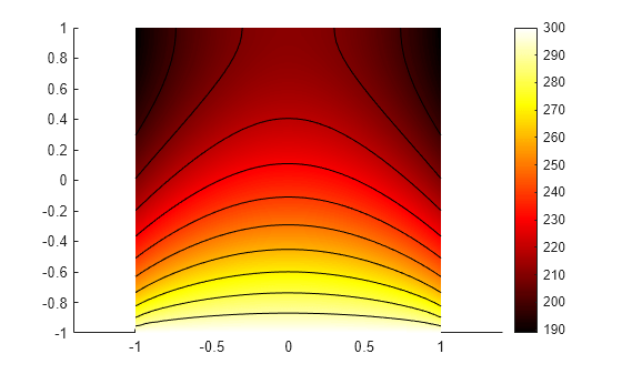
Interpolate the resulting temperatures to a grid covering the central portion of the geometry, for x and y from -0.5 to 0.5.

v = linspace(-0.5,0.5,11);
[X,Y] = meshgrid(v);

Tintrp = interpolateTemperature(R,X,Y);

Reshape the Tintrp vector and plot the resulting temperatures.

Tintrp = reshape(Tintrp,size(X));

figure
contourf(X,Y,Tintrp)
colormap(hot)
colorbar
axis equal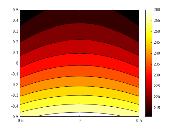

Alternatively, you can specify the grid by using a matrix of query points.

querypoints = [X(:),Y(:)]';
Tintrp = interpolateTemperature(R,querypoints);

Interpolate Temperature for a 3-D Steady-State Thermal Problem

Create an femodel object for steady-state thermal analysis and include a block geometry into the model.

model = femodel(AnalysisType="thermalSteady", ...
                Geometry="Block.stl");

Plot the geometry.

pdegplot(model.Geometry,FaceLabels="on",FaceAlpha=0.5)
title("Copper block, cm")

Assuming that this is a copper block, the thermal conductivity of the block is approximately 4 W/(cm*K).

model.MaterialProperties = ...
    materialProperties(ThermalConductivity=4);

Apply a constant temperature of 373 K to the left side of the block (edge 1) and a constant temperature of 573 K at the right side of the block.

model.FaceBC(1) = faceBC(Temperature=373);
model.FaceBC(3) = faceBC(Temperature=573);

Apply a heat flux boundary condition to the bottom of the block.

model.FaceLoad(4) = faceLoad(Heat=-20);

Mesh the geometry and solve the problem.

model = generateMesh(model);
R = solve(model)

R = 
  SteadyStateThermalResults with properties:

    Temperature: [12822×1 double]
     XGradients: [12822×1 double]
     YGradients: [12822×1 double]
     ZGradients: [12822×1 double]
           Mesh: [1×1 FEMesh]

The solver finds the values of temperatures and temperature gradients at the nodal locations. To access these values, use results.Temperature, results.XGradients, and so on. For example, plot temperatures at nodal locations.

pdeplot3D(R.Mesh,ColorMapData=R.Temperature)

Create a grid specified by x, y, and z coordinates and interpolate temperatures to the grid.

[X,Y,Z] = meshgrid(1:16:100,1:6:20,1:7:50);

Tintrp = interpolateTemperature(R,X,Y,Z);

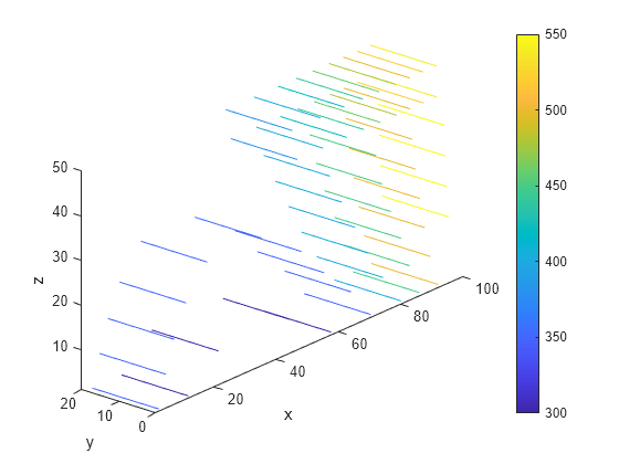
Create a contour slice plot for fixed values of the y coordinate.

Tintrp = reshape(Tintrp,size(X));
figure
contourslice(X,Y,Z,Tintrp,[],1:6:20,[])
xlabel("x")
ylabel("y")
zlabel("z")
xlim([1,100])
ylim([1,20])
zlim([1,50])
axis equal
view(-50,22)
colorbar

Alternatively, you can specify the grid by using a matrix of query points.

querypoints = [X(:),Y(:),Z(:)]';
Tintrp = interpolateTemperature(R,querypoints);

Create a contour slice plot for four fixed values of the z coordinate.

Tintrp = reshape(Tintrp,size(X));
figure
contourslice(X,Y,Z,Tintrp,[],[],1:7:50)
xlabel("x")
ylabel("y")
zlabel("z")
xlim([1,100])
ylim([1,20])
zlim([1,50])
axis equal
view(-50,22)
colorbar

Temperatures at Convective Boundary

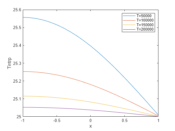
Solve a 2-D transient heat transfer problem on a square domain and compute temperatures at the convective boundary.

Create and plot a square geometry.

g = @squareg;
pdegplot(g,EdgeLabels="on")
xlim([-1.1,1.1])
ylim([-1.1,1.1])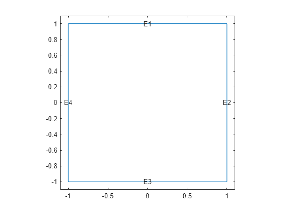

Create an femodel object for transient thermal analysis and include the geometry into the model.

model = femodel(AnalysisType="thermalTransient", ...
                Geometry=g);

Assign the following thermal properties:

• Thermal conductivity is 100 W/(m*C)

• Mass density is 7800 kg/m^3

• Specific heat is 500 J/(kg*C)

model.MaterialProperties = ...
    materialProperties(ThermalConductivity=100,...
                       MassDensity=7800,...
                       SpecificHeat=500);

Apply a convection boundary condition on the right edge.

model.EdgeLoad(2) = ...
    edgeLoad(ConvectionCoefficient=5000,...
             AmbientTemperature=25);

Set the initial conditions: uniform room temperature across domain and higher temperature on the left edge.

model.FaceIC = faceIC(Temperature=25);
model.EdgeIC(4) = edgeIC(Temperature=100);

Generate a mesh and solve the problem using 0:1000:200000 as a vector of times.

model = generateMesh(model);
tlist = 0:1000:200000;
R = solve(model,tlist);

Define a line at convection boundary and compute temperature gradients across that line.

X = -1:0.1:1;
Y = ones(size(X));
Tintrp = interpolateTemperature(R,X,Y,1:length(tlist));

Plot the interpolated temperature Tintrp along the x axis for the following values from the time interval tlist.

figure
t = 51:50:201;
p = gobjects(size(t));
for i = 1:numel(t)
  p(i) = plot(X,Tintrp(:,t(i)), ...
      DisplayName="T="+tlist(t(i)));
  hold on
end
legend(p)
xlabel("x")
ylabel("Tintrp")

Input Arguments

thermalresults — Solution of thermal problem

SteadyStateThermalResults object | TransientThermalResults object

Solution of thermal problem, specified as a SteadyStateThermalResults object or a TransientThermalResults object. Create thermalresults using solve.

xq — x-coordinate query points

real array

x-coordinate query points, specified as a real array. interpolateTemperature evaluates temperatures at the 2-D coordinate points [xq(i),yq(i)] or at the 3-D coordinate points [xq(i),yq(i),zq(i)]. So xq, yq, and (if present) zq must have the same number of entries.

interpolateTemperature converts query points to column vectors xq(:), yq(:), and (if present) zq(:). It returns temperatures in the form of a column vector of the same size. To ensure that the dimensions of the returned solution is consistent with the dimensions of the original query points, use reshape. For example, use Tintrp = reshape(Tintrp,size(xq)).

Data Types: double

yq — y-coordinate query points

real array

y-coordinate query points, specified as a real array. interpolateTemperature evaluates temperatures at the 2-D coordinate points [xq(i),yq(i)] or at the 3-D coordinate points [xq(i),yq(i),zq(i)]. So xq, yq, and (if present) zq must have the same number of entries. Internally, interpolateTemperature converts query points to the column vector yq(:).

Data Types: double

zq — z-coordinate query points

real array

z-coordinate query points, specified as a real array. interpolateTemperature evaluates temperatures at the 3-D coordinate points [xq(i),yq(i),zq(i)]. So xq, yq, and zq must have the same number of entries. Internally, interpolateTemperature converts query points to the column vector zq(:).

Data Types: double

querypoints — Query points

real matrix

Query points, specified as a real matrix with either two rows for 2-D geometry, or three rows for 3-D geometry. interpolateTemperature evaluates temperatures at the coordinate points querypoints(:,i), so each column of querypoints contains exactly one 2-D or 3-D query point.

Example: For 2-D geometry, querypoints = [0.5,0.5,0.75,0.75; 1,2,0,0.5]

Data Types: double

iT — Time indices

vector of positive integers

Time indices, specified as a vector of positive integers. Each entry in iT specifies a time index.

Example: iT = 1:5:21 specifies every fifth time-step up to 21.

Data Types: double

Output Arguments

Tintrp — Temperatures at query points

array

Temperatures at query points, returned as an array. For query points that are outside the geometry, Tintrp = NaN.

Version History

Introduced in R2017a