interpolateElectricFlux
Interpolate electric flux density in electrostatic result at arbitrary spatial locations
Syntax
Description
Dintrp = interpolateElectricFlux(electrostaticresults,xq,yq)xq and yq.
Dintrp = interpolateElectricFlux(electrostaticresults,querypoints)querypoints.
Examples
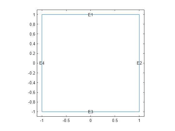
Create a square geometry and plot it with the edge labels.
R1 = [3,4,-1,1,1,-1,1,1,-1,-1]';
g = decsg(R1,'R1',('R1')');
pdegplot(g,EdgeLabels="on")
xlim([-1.1 1.1])
ylim([-1.1 1.1])
Create an femodel object for electrostatic analysis and include the geometry into the model.
model = femodel(AnalysisType="electrostatic", ...
                Geometry=g);
Specify the vacuum permittivity in the SI system of units.
model.VacuumPermittivity = 8.8541878128E-12;
Specify the relative permittivity of the material.
model.MaterialProperties = ...
    materialProperties(RelativePermittivity=1);
Apply the voltage boundary conditions on the edges of the square.
model.EdgeBC([1 3]) = edgeBC(Voltage=0);
model.EdgeBC([2 4]) = edgeBC(Voltage=1000);
Specify the charge density for the entire geometry.
model.FaceLoad = faceLoad(ChargeDensity=5E-9);
Generate the mesh.
model = generateMesh(model);
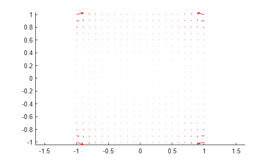
Solve the problem and plot the electric flux density.
R = solve(model);
pdeplot(R.Mesh,FlowData=[R.ElectricFluxDensity.Dx ...
                         R.ElectricFluxDensity.Dy])
axis equal
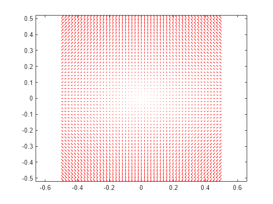
Interpolate the resulting electric flux density to a grid covering the central portion of the geometry, for x and y from -0.5 to 0.5.
v = linspace(-0.5,0.5,51);
[X,Y] = meshgrid(v);

Dintrp = interpolateElectricFlux(R,X,Y)
Dintrp =
  FEStruct with properties:

    Dx: [2601×1 double]
    Dy: [2601×1 double]
Reshape Dintrp.Dx and Dintrp.Dy and plot the resulting electric flux density.
DintrpX = reshape(Dintrp.Dx,size(X));
DintrpY = reshape(Dintrp.Dy,size(Y));

figure
quiver(X,Y,DintrpX,DintrpY,Color="red")
axis equal
Alternatively, you can specify the grid by using a matrix of query points.
querypoints = [X(:),Y(:)]';
Dintrp = interpolateElectricFlux(R,querypoints);
Create an femodel object for electrostatic analysis and include a geometry of a plate with a hole into the model.
model = femodel(AnalysisType="electrostatic", ...
                Geometry="PlateHoleSolid.stl");
Plot the geometry.
pdegplot(model.Geometry,FaceLabels="on",FaceAlpha=0.3)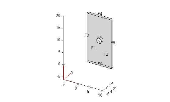
Specify the vacuum permittivity in the SI system of units.
model.VacuumPermittivity = 8.8541878128E-12;
Specify the relative permittivity of the material.
model.MaterialProperties = ...
    materialProperties(RelativePermittivity=1);
Specify the charge density for the entire geometry.
model.CellLoad = cellLoad(ChargeDensity=5E-9);
Apply the voltage boundary conditions on the side faces and the face bordering the hole.
model.FaceBC(3:6) = faceBC(Voltage=0);
model.FaceBC(7) = faceBC(Voltage=1000);
Generate the mesh.
model = generateMesh(model);
Solve the problem.
R = solve(model)
R =
  ElectrostaticResults with properties:

      ElectricPotential: [4747×1 double]
          ElectricField: [1×1 FEStruct]
    ElectricFluxDensity: [1×1 FEStruct]
                   Mesh: [1×1 FEMesh]
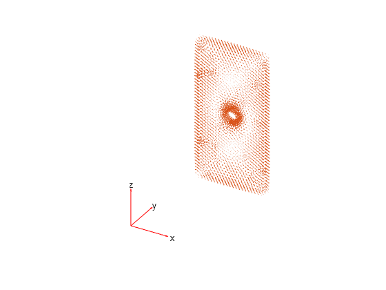
Plot the electric flux density.
pdeplot3D(R.Mesh,FlowData=[R.ElectricFluxDensity.Dx ...
                           R.ElectricFluxDensity.Dy ...
                           R.ElectricFluxDensity.Dz])
Interpolate the resulting electric flux density to a grid covering the central portion of the geometry, for x, y, and z.
x = linspace(3,7,7);
y = linspace(0,1,7);
z = linspace(8,12,7);
[X,Y,Z] = meshgrid(x,y,z);

Dintrp = interpolateElectricFlux(R,X,Y,Z);
Reshape Dintrp.Dx, Dintrp.Dy, and Dintrp.Dz.
DintrpX = reshape(Dintrp.Dx,size(X));
DintrpY = reshape(Dintrp.Dy,size(Y));
DintrpZ = reshape(Dintrp.Dz,size(Z));
Plot the resulting electric flux density.
figure
quiver3(X,Y,Z,DintrpX,DintrpY,DintrpZ,Color="red")
view([10 10])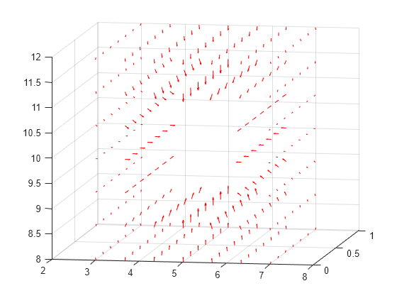
Input Arguments
Output Arguments
Version History
Introduced in R2021a