ポートフォリオ最適化問題に対する二次計画法、ソルバーベース

R2026b

この例では、quadprog の内点二次計画法アルゴリズムを使用して、ポートフォリオ最適化の問題を解く方法を示します。関数 quadprog は、Optimization Toolbox™ に含まれています。

この例の問題を定義する行列は高密度ですが、quadprog の内点法アルゴリズムでは、問題の行列にあるスパースを活用して速度を上げることもできます。スパースの例については、内点法アルゴリズムを使った大規模なスパース二次計画法を参照してください。

二次モデル

$n$ 種類の資産があるとします。資産 $i$ の収益率は、期待値が $m_{i}$ の確率変数です。問題は、指定された最小期待収益率を条件として、リスクを最小限にするには、どの割合 $x_{i}$ で各資産 $i$ に投資するかを求めることです。

$C$ は資産収益率の共分散行列を示すとします。

従来の平均分散モデルは、以下の測定でポートフォリオリスクを最小化し、

$\frac{1}{2} x^{T} C x$

これは一連の制約に従います。

期待される収益は、投資家が望むポートフォリオの最小期待収益率 $r$ を下回ってはなりません。

$\sum_{i = 1}^{n} m_{i} x_{i} \geq r,$

投資割合 $x_{i}$ の合計は 1 にならなければなりません。

$\sum_{i = 1}^{n} x_{i} = 1,$

そして、割合 (またはパーセント) は、0 と 1 の間の数でなければなりません。

$0 \leq x_{i} \leq 1, i = 1 \dots n .$

ポートフォリオリスクを最小限に抑えるという目的関数は二次で制約は線形であるため、最適化問題は最終的に二次計画、つまり QP となります。

225 資産問題

ここで、225 資産をもつ QP を解いてみます。データセットは、OR ライブラリ [Chang, T.-J., Meade, N., Beasley, J.E. and Sharaiha, Y.M., "Heuristics for cardinality constrained portfolio optimisation" Computers & Operations Research 27 (2000) 1271-1302] からの引用です。

データセットを読み込み、制約を quadprog で期待する形式に設定します。このデータセットでは、収益率 $m_{i}$ は –0.008489 ～ 0.003971 の範囲にあります。その中から望ましい収益 $r$ 、たとえば 0.002 (0.2%) を選択します。

MAT ファイルに保存されているデータセットを読み込みます。

load("port5.mat","Correlation","stdDev_return","mean_return")

共分散行列を相関行列から計算します。

Covariance = Correlation .* (stdDev_return * stdDev_return');
nAssets = numel(mean_return); r = 0.002;     % number of assets and desired return
Aeq = ones(1,nAssets); beq = 1;              % equality Aeq*x = beq
Aineq = -mean_return'; bineq = -r;           % inequality Aineq*x <= bineq
lb = zeros(nAssets,1); ub = ones(nAssets,1); % bounds lb <= x <= ub
c = zeros(nAssets,1);                        % objective has no linear term; set it to zero

quadprog の内点法アルゴリズムの選択

内点法アルゴリズムを使用して QP を解くために、Algorithm オプションを "interior-point-convex" に設定します。

options = optimoptions("quadprog",Algorithm="interior-point-convex");

225 資産問題の解法

ここでは、いくつかの追加オプションを設定し、ソルバー quadprog を呼び出します。

追加オプションを設定します。反復表示をオンにして、最適性に関する終了許容誤差を小さくします。

options = optimoptions(options,Display="iter",TolFun=1e-10);

ソルバーを呼び出し、時計時間を測定します。

tic
[x1,fval1] = quadprog(Covariance,c,Aineq,bineq,Aeq,beq,lb,ub,[],options);

 Iter            Fval  Primal Infeas    Dual Infeas  Complementarity   Wall-Clock Time  
    0    2.384401e+01   2.253410e+02   1.337381e+00     1.000000e+00      0.010899 sec  
    1    1.338822e-03   7.394864e-01   4.388791e-03     1.038098e-02      0.013597 sec  
    2    1.186079e-03   6.443975e-01   3.824446e-03     8.727381e-03      0.016201 sec  
    3    5.923977e-04   2.730703e-01   1.620650e-03     1.174211e-02      0.017235 sec  
    4    5.354880e-04   5.303581e-02   3.147632e-04     1.549549e-02      0.018875 sec  
    5    5.181994e-04   2.651791e-05   1.573816e-07     2.848171e-04      0.020082 sec  
    6    5.066191e-04   9.285375e-06   5.510794e-08     1.041224e-04      0.021072 sec  
    7    3.923090e-04   7.619855e-06   4.522322e-08     5.536006e-04      0.022048 sec  
    8    3.791545e-04   1.770065e-06   1.050519e-08     1.382075e-04      0.023050 sec  
    9    2.923749e-04   8.850312e-10   5.252599e-12     3.858983e-05      0.023977 sec  
   10    2.277722e-04   4.431702e-13   2.627914e-15     6.204101e-06      0.024911 sec  
   11    1.992243e-04   2.229120e-16   2.127959e-18     4.391483e-07      0.025887 sec  
   12    1.950468e-04   3.339343e-16   1.456847e-18     1.429441e-08      0.028161 sec  
   13    1.949141e-04   3.330669e-16   1.239159e-18     9.731942e-10      0.029922 sec  
   14    1.949121e-04   8.886121e-16   6.938894e-18     2.209702e-12      0.031055 sec  

Minimum found that satisfies the constraints.

Optimization completed because the objective function is non-decreasing in 
feasible directions, to within the value of the optimality tolerance,
and constraints are satisfied to within the value of the constraint tolerance.

<stopping criteria details>

toc

Elapsed time is 0.049400 seconds.

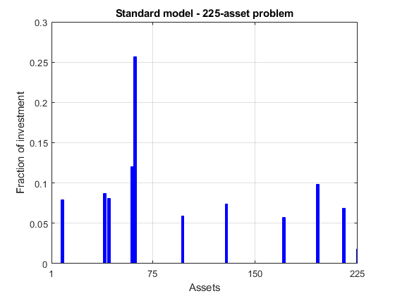
結果をプロットします。

plotPortfDemoStandardModel(x1)

$Bar chart of optimal investment fractions for the 225-asset standard model, showing most weight concentrated in a few assets$

グループ制約付き 225 資産問題

資産 1 ～ 75、76 ～ 150、151 ～ 225 のそれぞれに投資金額の 30% を投資することを要求する制約をモデルグループに追加します。これらの資産グループのそれぞれは、たとえば技術、自動車、医薬品など産業が異なることもあります。この新しい要件を含む制約は、以下のとおりです。

$\sum_{i = 1}^{75} x_{i} \geq 0.3,$

$\sum_{i = 76}^{150} x_{i} \geq 0.3,$

$\sum_{i = 151}^{225} x_{i} \geq 0.3 .$

既存の等式にグループ制約を追加します。

Groups = blkdiag(ones(1,nAssets/3),ones(1,nAssets/3),ones(1,nAssets/3));
Aineq = [Aineq; -Groups];         % convert to <= constraint
bineq = [bineq; -0.3*ones(3,1)];  % by changing signs

ソルバーを呼び出し、時計時間を測定します。

tic
[x2,fval2] = quadprog(Covariance,c,Aineq,bineq,Aeq,beq,lb,ub,[],options);

 Iter            Fval  Primal Infeas    Dual Infeas  Complementarity   Wall-Clock Time  
    0    2.384401e+01   4.464410e+02   1.337324e+00     1.000000e+00      0.014846 sec  
    1    1.346872e-03   1.474737e+00   4.417606e-03     3.414918e-02      0.018766 sec  
    2    1.190113e-03   1.280566e+00   3.835962e-03     2.934585e-02      0.019984 sec  
    3    5.990845e-04   5.560762e-01   1.665738e-03     1.320038e-02      0.021216 sec  
    4    3.890097e-04   2.780381e-04   8.328691e-07     7.287370e-03      0.022435 sec  
    5    3.887354e-04   1.480950e-06   4.436215e-09     4.641988e-05      0.023652 sec  
    6    3.387787e-04   8.425389e-07   2.523843e-09     2.578178e-05      0.024865 sec  
    7    3.089240e-04   2.707587e-07   8.110632e-10     9.217509e-06      0.026066 sec  
    8    2.639458e-04   6.586817e-08   1.973095e-10     6.509001e-06      0.027276 sec  
    9    2.252657e-04   2.225507e-08   6.666551e-11     6.783212e-06      0.028496 sec  
   10    2.105838e-04   5.811527e-09   1.740855e-11     1.967570e-06      0.029699 sec  
   11    2.024362e-04   4.129834e-12   1.237133e-14     5.924109e-08      0.030909 sec  
   12    2.009704e-04   3.787335e-15   1.441446e-17     6.354389e-10      0.032113 sec  
   13    2.009650e-04   6.665675e-16   6.938894e-18     1.889136e-13      0.033325 sec  

Minimum found that satisfies the constraints.

Optimization completed because the objective function is non-decreasing in 
feasible directions, to within the value of the optimality tolerance,
and constraints are satisfied to within the value of the constraint tolerance.

<stopping criteria details>

toc

Elapsed time is 0.051104 seconds.

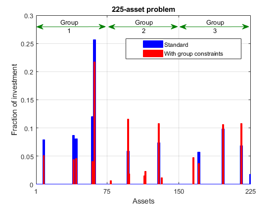
結果を前の問題の結果に重ね合わせてプロットします。

plotPortfDemoGroupModel(x1,x2);

Bar chart comparing standard and group-constrained portfolio allocations across 225 assets, showing more even distribution with group constraints

これまでの結果の概要

2 番目の棒グラフを見ると、このポートフォリオは、グループ制約を追加したことにより、最初のポートフォリオと比べて 3 つの資産グループへの分配がより均一であることがわかります。また、この多様性により、目的関数 (両実行の反復表示で最後の反復に "f(x)" が付いている列を参照) で測定したところ、リスクがわずかに増加する結果となりました。

乱数データを使用した 1000 資産問題

quadprog の内点法アルゴリズムがより大きな問題でどのような動作を行うかを示すため、1000 資産のランダムに生成されたデータセットを使用します。MATLAB® で関数 gallery を使用して、ランダム相関行列 (対称、半正定値、対角要素が 1) を生成します。

再現性が必要な場合は、乱数ストリームをリセットします。

rng(0,"twister");
nAssets = 1000; % desired number of assets

–0.1 ～ 0.4 の収益の平均を生成します。

a = -0.1; b = 0.4;
mean_return = a + (b-a).*rand(nAssets,1);

0.08 ～ 0.6 の収益の標準偏差を生成します。

a = 0.08; b = 0.6;
stdDev_return = a + (b-a).*rand(nAssets,1);
% Correlation matrix, generated using Correlation = gallery("randcorr",nAssets).
% (Generating a correlation matrix of this size takes a while, so we load
% a pre-generated one instead.)
load("correlationMatrixDemo.mat","Correlation");
% Calculate covariance matrix from correlation matrix.
Covariance = Correlation .* (stdDev_return * stdDev_return');

ランダムに作成された 1000 資産問題の定義と解法

それでは、標準的な QP 問題 (ここではグループ制約なし) を定義し、解いてみます。

r = 0.15;                                     % desired return
Aeq = ones(1,nAssets); beq = 1;               % equality Aeq*x = beq
Aineq = -mean_return'; bineq = -r;            % inequality Aineq*x <= bineq
lb = zeros(nAssets,1); ub = ones(nAssets,1);  % bounds lb <= x <= ub
c = zeros(nAssets,1);                         % objective has no linear term; set it to zero

ソルバーを呼び出し、時計時間を測定します。

tic
x3 = quadprog(Covariance,c,Aineq,bineq,Aeq,beq,lb,ub,[],options);

 Iter            Fval  Primal Infeas    Dual Infeas  Complementarity   Wall-Clock Time  
    0    7.083800e+01   1.142266e+03   1.610094e+00     1.000000e+00      0.032607 sec  
    1    5.603619e-03   7.133717e+00   1.005541e-02     9.857295e-02      0.052084 sec  
    2    1.076070e-04   3.566858e-03   5.027704e-06     9.761758e-03      0.072225 sec  
    3    1.068230e-04   2.513041e-06   3.542285e-09     8.148386e-06      0.097277 sec  
    4    7.257177e-05   1.230928e-06   1.735068e-09     3.979480e-06      0.124965 sec  
    5    3.610589e-05   2.634706e-07   3.713779e-10     1.175001e-06      0.150548 sec  
    6    2.077811e-05   2.562892e-08   3.612553e-11     5.617206e-07      0.179925 sec  
    7    1.611590e-05   4.711751e-10   6.641535e-13     5.652911e-08      0.194411 sec  
    8    1.491953e-05   4.926282e-12   6.940520e-15     2.427880e-09      0.210023 sec  
    9    1.477930e-05   1.317835e-13   1.852562e-16     2.454705e-10      0.411949 sec  
   10    1.476910e-05   8.049117e-16   9.619336e-19     2.786060e-11      0.446714 sec  

Minimum found that satisfies the constraints.

Optimization completed because the objective function is non-decreasing in 
feasible directions, to within the value of the optimality tolerance,
and constraints are satisfied to within the value of the constraint tolerance.

<stopping criteria details>

toc

Elapsed time is 0.466687 seconds.

まとめ

この例では、ポートフォリオ最適化問題において quadprog の内点法アルゴリズムを使用する方法を説明し、さまざまなサイズの二次問題におけるアルゴリズム実行時間を示します。

特に Financial Toolbox™ でのポートフォリオ最適化用に設計された機能を使用すると、より詳細な分析が可能です。

参考

混合整数二次計画法ポートフォリオ最適化問題: ソルバーベース