範囲制約付きの二次計画法: 問題ベース

この例では、拡張可能な範囲制約付き問題を二次目的関数により定式化して解く方法を示します。この例では、複数のアルゴリズムを使用して解の挙動を示します。問題には任意の個数の変数を含めることができます。変数の個数はスケールです。この例のソルバーベースのバージョンについては、範囲に制約のある二次の最小化を参照してください。

目的関数は問題変数の個数 n の関数であり、次のようになります。

$$2\sum _{i=1}^n{x}_i^2-2\sum _{i=1}^{n-1}{x}_i{x}_{i+1}-2x_1-2x_n.$$

問題の作成

400 個の成分がある、x という名前の問題変数を作成します。また、目的関数用に objec という名前の式を作成します。各変数の下限を 0、上限を 0.9 に設定します。ただし、$x_n$ は非有界が許可されます。

n = 400;
x = optimvar("x",n,LowerBound=0,UpperBound=0.9);
x(n).LowerBound = -Inf;
x(n).UpperBound = Inf;
prevtime = 1:n-1;
nexttime = 2:n;
objec = 2*sum(x.^2) - 2*sum(x(nexttime).*x(prevtime)) - 2*x(1) - 2*x(end);

qprob という名前の最適化問題を作成します。目的関数を問題に含めます。

qprob = optimproblem(Objective=objec);

quadprog の "trust-region-reflective" アルゴリズムと表示なしを指定するオプションを作成します。範囲のほぼ中央にある初期点を作成します。

opts = optimoptions("quadprog",Algorithm="trust-region-reflective",Display="off");
x0 = 0.5*ones(n,1);
x00 = struct("x",x0);

問題を解いて解を確認する

問題を解きます。

[sol,qfval,qexitflag,qoutput] = solve(qprob,x00,Options=opts);

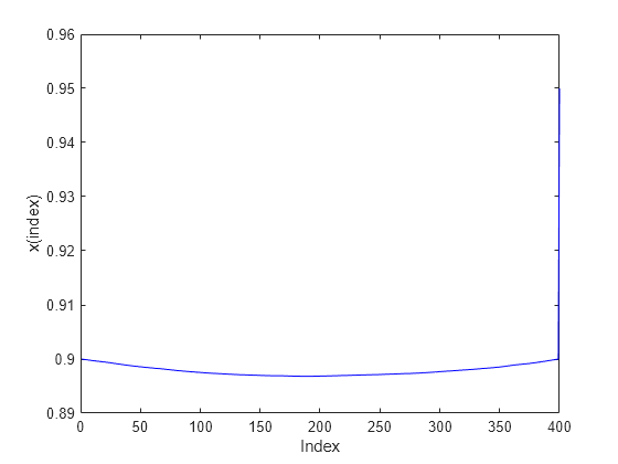
解をプロットします。

plot(sol.x,"b-")
xlabel("Index")
ylabel("x(index)")

終了フラグ、反復回数、および共役勾配の反復回数をレポートします。

fprintf("Exit flag = %d, iterations = %d, cg iterations = %d\n",...
    double(qexitflag),qoutput.iterations,qoutput.cgiterations)

Exit flag = 3, iterations = 20, cg iterations = 1813

共役勾配の反復が多数ありました。

効率を向上させるためのオプションの調整

SubproblemAlgorithm オプションを "factorization" に設定して、共役勾配の反復回数を減らします。このオプションにより、時間のかかる内部的な解法をソルバーが使用することで、共役勾配のステップが削減されます。このケースでは全体的に正味時間が節約されます。

opts.SubproblemAlgorithm = "factorization";
[sol2,qfval2,qexitflag2,qoutput2] = solve(qprob,x00,Options=opts);
fprintf("Exit flag = %d, iterations = %d, cg iterations = %d\n",...
    double(qexitflag2),qoutput2.iterations,qoutput2.cgiterations)

Exit flag = 3, iterations = 10, cg iterations = 0

反復回数と共役勾配の反復回数が少なくなりました。

"interior-point" の解との解の比較

これらの解を、既定の "interior-point" アルゴリズムを使用して得られるものと比較します。"interior-point" アルゴリズムは初期点を使用しないので、x00 を solve に渡しません。

opts = optimoptions("quadprog",Algorithm="interior-point-convex",Display="off");
[sol3,qfval3,qexitflag3,qoutput3] = solve(qprob,Options=opts);
fprintf("Exit flag = %d, iterations = %d, cg iterations = %d\n",...
    double(qexitflag3),qoutput3.iterations,0)

Exit flag = 1, iterations = 8, cg iterations = 0

middle = floor(n/2);
fprintf("The three solutions are slightly different.\nThe middle component is %f, %f, or %f.\n",...
    sol.x(middle),sol2.x(middle),sol3.x(middle))

The three solutions are slightly different.
The middle component is 0.897338, 0.898801, or 0.857389.

fprintf("The relative norm of sol - sol2 is %f.\n",norm(sol.x-sol2.x)/norm(sol.x))

The relative norm of sol - sol2 is 0.001116.

fprintf("The relative norm of sol2 - sol3 is %f.\n",norm(sol2.x-sol3.x)/norm(sol2.x))

The relative norm of sol2 - sol3 is 0.036007.

fprintf("The three objective function values are %f, %f, and %f.\n" ...
    +"The ''interior-point'' algorithm is slightly less accurate.",qfval,qfval2,qfval3)

The three objective function values are -1.985000, -1.985000, and -1.984963.
The ''interior-point'' algorithm is slightly less accurate.

参考

トピック

• 範囲に制約のある二次の最小化
• 問題ベースの最適化ワークフロー