大規模なスパース二次計画法、問題ベース

この例は、スパース問題を解くときにスパース演算を使用することの価値を示しています。行列は n 行です。大きい値の n と、いくつかの非ゼロの対角帯を選択します。n 行 n 列の非スパース行列は使用可能なメモリをすべて使用することがありますが、スパース行列は問題を起こしません。

問題は以下の制約に従って x'*H*x/2 + f'*x を最小化することです。

x(1) + x(2) + ... + x(n) <= 0,

ここで、f = [-1;-2;-3;...;-n]、H はスパース対称帯行列です。

スパース二次行列の作成

14 を主対角に置いたシフトにより、ベクトル [3,6,2,14,2,6,3] のシフトに基づいて対称循環行列 H を作成します。行列は n 行 n 列にします。ここで、n = 30,000 です。

n = 3e4;
H2 = speye(n);
H = 3*circshift(H2,-3,2) + 6*circshift(H2,-2,2) + 2*circshift(H2,-1,2)...
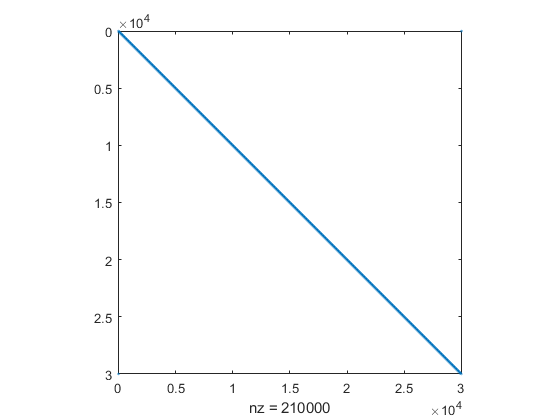
    + 14*H2 + 2*circshift(H2,1,2) + 6*circshift(H2,2,2) + 3*circshift(H2,3,2);

スパース行列の構造を表示します。

spy(H)

最適化変数と問題の作成

最適化変数 x と問題 qprob を作成します。

x = optimvar('x',n);
qprob = optimproblem;

目的関数と制約を作成します。目的関数と制約を qprob に設定します。

f = 1:n;
obj = 1/2*x'*H*x - f*x;
qprob.Objective = obj;
cons = sum(x) <= 0;
qprob.Constraints = cons;

問題を解く

既定の 'interior-point-convex' アルゴリズムとスパース線形代数を使用して、二次計画問題を解きます。ソルバーが途中で停止しないように、StepTolerance オプションを 0 に設定します。

options = optimoptions('quadprog','Algorithm','interior-point-convex',...
    'LinearSolver','sparse','StepTolerance',0);
[sol,fval,exitflag,output,lambda] = solve(qprob,'Options',options);

Minimum found that satisfies the constraints.

Optimization completed because the objective function is non-decreasing in 
feasible directions, to within the value of the optimality tolerance,
and constraints are satisfied to within the value of the constraint tolerance.

<stopping criteria details>

解の検証

目的関数の値、反復回数、および線形不等式制約に関連付けられたラグランジュ乗数を表示します。

fprintf('The objective function value is %d.\nThe number of iterations is %d.\nThe Lagrange multiplier is %d.\n',...
    fval,output.iterations,lambda.Constraints)

The objective function value is -3.133073e+10.
The number of iterations is 7.
The Lagrange multiplier is 1.500050e+04.

制約を評価して、解が境界上であることを確認します。

fprintf('The linear inequality constraint sum(x) has value %d.\n',sum(sol.x))

The linear inequality constraint sum(x) has value 7.599738e-09.

解の構成要素の合計は 0 で、許容誤差の範囲内です。

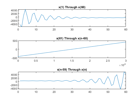
解 x には 3 つの領域、最初の部分、最後の部分、および解の大半を占めるほぼ線形の部分があります。3 つの領域をプロットします。

subplot(3,1,1)
plot(sol.x(1:60))
title('x(1) Through x(60)')
subplot(3,1,2)
plot(sol.x(61:n-60))
title('x(61) Through x(n-60)')
subplot(3,1,3)
plot(sol.x(n-59:n))
title('x(n-59) Through x(n)')

関連するトピック

• 内点法アルゴリズムを使った大規模なスパース二次計画法
• 問題ベースの最適化ワークフロー