GNSS シミュレーションの概要

全地球航法衛星システム (GNSS) シミュレーションでは、受信機の位置推定を生成します。これらの受信機の位置推定は、GPS と GNSS のセンサー モデルからgpsSensorオブジェクトおよびgnssSensorオブジェクトとして得られます。精度低下率の出力を使用して gnssSensor の位置推定のステータスを監視し、使用可能な衛星の数を比較します。

シミュレーション パラメーター

GNSS シミュレーションで使用するパラメーターを指定します。

• GNSS 受信機のサンプリング レート

• ローカル ナビゲーション基準座標系

• 地球上の緯度、経度、高度 (LLA) 座標系における位置

• シミュレートするサンプル数

Fs = 1;
refFrame = "NED";
lla0 = [42.2825 -71.343 53.0352];
N = 100;

固定センサーの軌跡を作成します。

pos = zeros(N, 3);
vel = zeros(N, 3);
time = (0:N-1) ./ Fs;

センサー モデルの作成

それぞれ同じ初期パラメーターを使用して GNSS シミュレーション オブジェクト gpsSensor と gnssSensor を作成します。

gps = gpsSensor("SampleRate", Fs, "ReferenceLocation", lla0, ...
    "ReferenceFrame", refFrame);

gnss = gnssSensor("SampleRate", Fs, "ReferenceLocation", lla0, ...
    "ReferenceFrame", refFrame);

gpsSensor を使用したシミュレーション

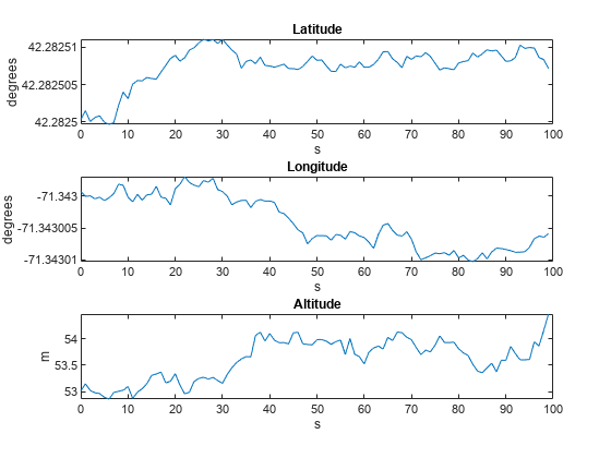
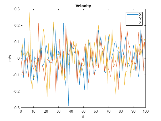
GPS センサーを使用して固定受信機からの出力を生成します。LLA 座標系の位置と各方向の速度を可視化します。

% Generate outputs.
[llaGPS, velGPS] = gps(pos, vel);

% Visualize position.
figure
subplot(3, 1, 1)
plot(time, llaGPS(:,1))
title('Latitude')
ylabel('degrees')
xlabel('s')
subplot(3, 1, 2)
plot(time, llaGPS(:,2))
title('Longitude')
ylabel('degrees')
xlabel('s')
subplot(3, 1, 3)
plot(time, llaGPS(:,3))
title('Altitude')
ylabel('m')
xlabel('s')

% Visualize velocity.
figure
plot(time, velGPS)
title('Velocity')
legend('X', 'Y', 'Z')
ylabel('m/s')
xlabel('s')

gnssSensor を使用したシミュレーション

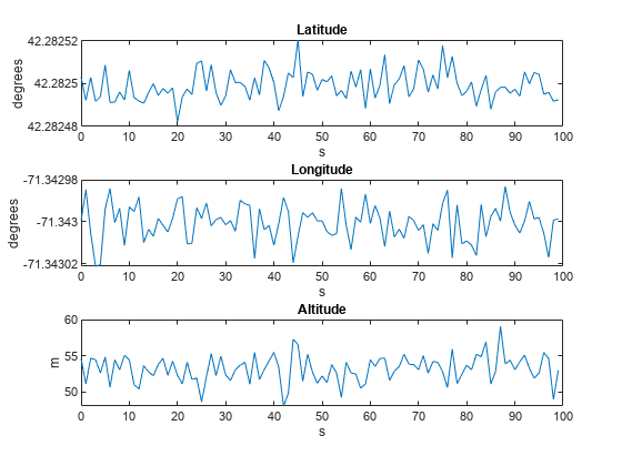
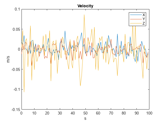
GNSS センサーを使用して固定受信機からの出力を生成します。位置と速度を可視化し、シミュレーションにおける違いを確認します。

% Generate outputs.
[llaGNSS, velGNSS] = gnss(pos, vel);

% Visualize positon.
figure
subplot(3, 1, 1)
plot(time, llaGNSS(:,1))
title('Latitude')
ylabel('degrees')
xlabel('s')
subplot(3, 1, 2)
plot(time, llaGNSS(:,2))
title('Longitude')
ylabel('degrees')
xlabel('s')
subplot(3, 1, 3)
plot(time, llaGNSS(:,3))
title('Altitude')
ylabel('m')
xlabel('s')

% Visualize velocity.
figure
plot(time, velGNSS)
title('Velocity')
legend('X', 'Y', 'Z')
ylabel('m/s')
xlabel('s')

精度低下率

gnssSensor オブジェクトのシミュレーションは、gpsSensor と比較して忠実度が高くなります。たとえば、gnssSensor オブジェクトでは、シミュレートした衛星の位置を使用して受信機の位置を推定します。これは、位置推定と共に水平精度低下率 (HDOP) と垂直精度低下率 (VDOP) をレポートできることを意味します。これらの値は、衛星の配置に基づく位置推定の正確さを示します。値が小さいほど正確な推定であることを示します。

% Set the RNG seed to reproduce results. 
rng('default')

% Specify the start time of the simulation.
initTime = datetime(2020, 4, 20, 18, 10, 0, "TimeZone", "America/New_York");

% Create the GNSS receiver model.
gnss = gnssSensor("SampleRate", Fs, "ReferenceLocation", lla0, ...
    "ReferenceFrame", refFrame, "InitialTime", initTime);

% Obtain the receiver status. 
[~, ~, status] = gnss(pos, vel);
disp(status(1))

      SatelliteAzimuth: [7x1 double]
    SatelliteElevation: [7x1 double]
                  HDOP: 1.1290
                  VDOP: 1.9035

シミュレーション全体における HDOP を表示します。HDOP の低下が見られます。これは、衛星の配置が変化したことを意味します。

hdops = vertcat(status.HDOP);

figure
plot(time, vertcat(status.HDOP))
title('HDOP')
ylabel('m')
xlabel('s')

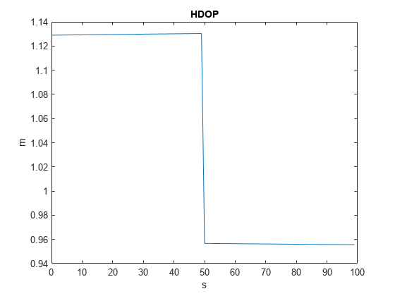
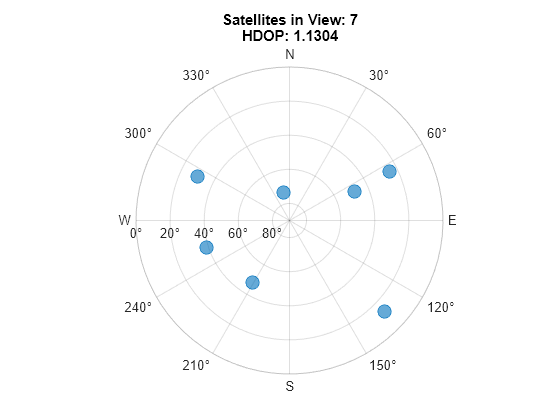
衛星の配置が変化していることを確認します。HDOP が低下したインデックスを調べ、それが視野内の衛星数の変化と対応しているかどうかを確認します。変数 numSats が 7 から 8 に増えています。

% Find expected sample index for a change in the
% number of satellites in view.
[~, satChangeIdx] = max(abs(diff(hdops)));

% Visualize the satellite geometry before the
% change in HDOP.
satAz = status(satChangeIdx).SatelliteAzimuth;
satEl = status(satChangeIdx).SatelliteElevation;
numSats = numel(satAz);
skyplot(satAz, satEl);
title(sprintf('Satellites in View: %d\nHDOP: %.4f', ...
    numSats, hdops(satChangeIdx)))

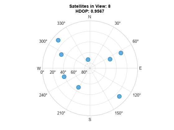
% Visualize the satellite geometry after the
% change in HDOP.
satAz = status(satChangeIdx+1).SatelliteAzimuth;
satEl = status(satChangeIdx+1).SatelliteElevation;
numSats = numel(satAz);
skyplot(satAz, satEl);
title(sprintf('Satellites in View: %d\nHDOP: %.4f', ...
    numSats, hdops(satChangeIdx+1)))

GNSS 受信機の位置推定をカルマン フィルターを使用して他のセンサー測定と組み合わせると、HDOP と VDOP の値を測定共分散行列で対角要素として使用できます。

% Convert HDOP and VDOP to a measurement covariance matrix.
hdop = status(1).HDOP;
vdop = status(1).VDOP;
measCov = diag([hdop.^2/2, hdop.^2/2, vdop.^2]);
disp(measCov)

    0.6373         0         0
         0    0.6373         0
         0         0    3.6233