Current Result - Optimization Solution

You can select from these views on the right-hand side (RHS) of the Optimization Output view under Current Result - Optimization Solution:

• Objective Slice Graphs — Shows cross-section plots of the objective function against each optimization variable in the problem at the point selected in the Optimization Results table.

• Objective Contour Plot — Shows the contours of the objective against any pair of control parameters at the run selected in the Optimization Results table.

• Constraint Slice Graphs — Shows the constraint functions at the selected operating point with the solution value.

• Constraint Summary Table — Displays the constraint values for the selected solution in the table.

• Free Variables Table — Displays the values of the optimization variables for the currently selected solution.

• Solution Information Table — Displays additional information about the optimization results.

The panel on the RHS of the view shows these additional details about what is visualized:

• Summary Information — Displays the optimization value and the lookup table value of the selected operating point.

• Current Operating Point — Displays the fixed-variable values at the selected operating point.

• Lookup Tables — Displays a list of lookup tables and the corresponding optimization results used to fill the lookup tables

• Current Result Evaluation — Toggle between displaying the Optimization Solution or the Lookup Tables Values in the graphs and tables on the RHS.

The default view of tables and graphs is dependent on the optimization type.

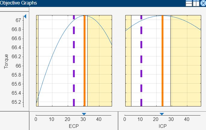
Objective Slice Graphs

To display the objective slice graph select in the toolbar.

The objective slice graphs display cross-section plots of the objective function against each optimization variable in the problem at the point selected in the Optimization Results table. The solution value is shown in orange, and lookup table value is in purple. For multiobjective optimization results, whether the Optimization Results table is displaying a solution slice or Pareto slice, the cell you select in the table is always displayed in the graphs.

The yellow areas indicate a region outside of a constraint tolerance, such as a boundary constraint exported from the Model Browser or any other optimization constraint. All constraint regions are displayed in yellow.

Use the right-click context menu to toggle constraint display and alter graph size.

Objective Contour Plot

The Objective Contours plot (click ) shows the contours of the objective against any pair of control parameters at the run selected in the Optimization Results table. The solution value is at the center of the orange cross-hairs, and the lookup table value is in purple. Yellow areas indicate a region outside of a constraint tolerance. This view helps explore objective functions visually to avoid local minima.

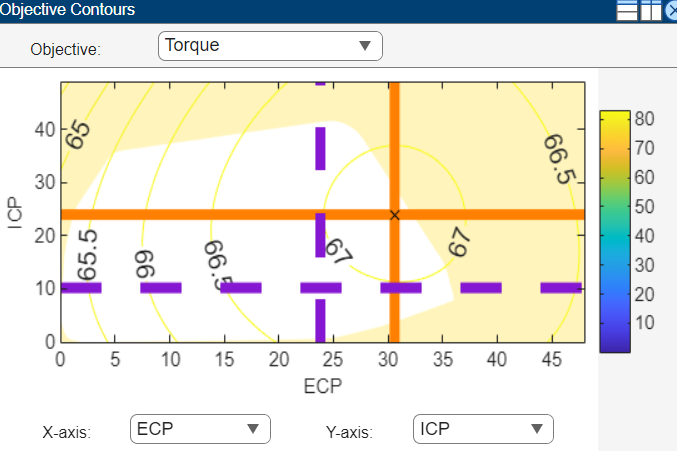
Select parameters to plot from the drop-down lists. If multiple objectives exist, select from the Objective drop-down list.

Use the right-click context menu to toggle constraint display, contour labels, fill contours, and color bar, and control other options.

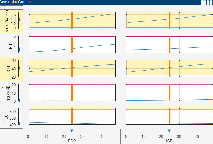
Constraint Slice Graphs

The Constraint Slice graphs (click ) show the constraint functions at the selected operating point with the solution value in orange. Click inside the tables to select solutions to display. Yellow areas on the graphs indicate a region outside a constraint tolerance, as shown in this figure.

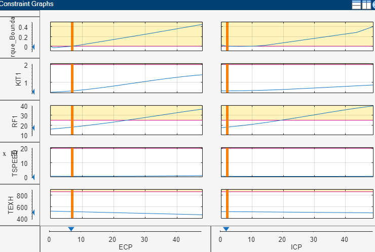
This example shows the constraint graphs of a selected run in the Torque_Optimization optimization from the Dual CAM gasoline engine with spark optimized during testing case study.

The blue line of the constraint graphs show how the Left Value of each output of a constraint depends on the optimization variables in the optimization. The Left Value is compared with a plot of the Right Value output on the same axes.

The red horizontal line indicates the Right Value. Because this value is an upper bound, the yellow region above the red line shows where the constraint is infeasible. Yellow is shown above the Right Value plus the tolerance — on many graphs, the distance is too small to see between the red line and the tolerance line. By default, this tolerance is taken from the optimization constraint tolerance. You can control the value used for this highlighting by selecting View > Edit Constraint Tolerance.

The vertical orange lines show the optimal values of the optimization variables. The intersection of these with the blue lines is marked with a blue triangle on the axes—this intersection is the Left Value at the optimal settings.

If a constraint is violated at the solution value, the Y axis is highlighted in yellow, as shown in this example. If constraint values are greater than the tolerance, the row is highlighted in yellow. By default, this tolerance is taken from the optimization constraint tolerance. You can control the value used for this highlighting by selecting View > Edit Constraint Tolerance.

Constraint Summary Table

The Constraint Summary (click ) view displays the constraint values for the selected solution in the table. Use this view to quickly determine if a solution meets all constraints. If there are many constraints, it is time-consuming to use the constraint graphs for verification. If you are using equality constraints or tight table gradient constraints, the graphs can appear entirely yellow. You can only see a feasible solution by looking at the Constraint Summary Table, shown in this figure.

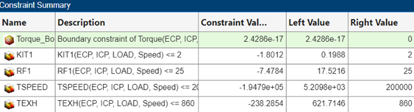
Constraints are active when the Left Value is within a tolerance of the Right Value. Active constraints are highlighted in green. Constraint values greater than the tolerance are highlighted in yellow. By default, this tolerance is taken from the optimization constraint tolerance. You can control the value used for this highlighting by selecting View > Edit Constraint Tolerance. These results should be checked as they might show that the optimization failed to find a solution within the constraint, or they might be within tolerance (very close to zero). Constraint values less than zero are within the constraint.

Constraints are evaluated as inequalities. For example, the RF1 constraint is expressed as RF1<=25. The Left Value represents the left side of the inequality at the optimal settings of the optimization variables, which is 15.1442. The Right Value indicates the upper bound, which is 25. The Constraint Value is the difference between the Left Value and the Right Value, showing the distance to the constraint edge.

Solution Information Table

The Solution Information table displays outputs of the fmincon algorithm for the currently selected solution. Hover the mouse pointer over the Exit message to see the whole exit message. For example, this message can tell you if an fmincon optimization run terminated because no feasible start point was found.

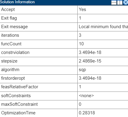
This table lists MBC specific exit flags.

Exit Flag	Description
11	Optimization stopped at a feasible solution.
12	Optimization stopped at an infeasible solution due to soft constraints.
13	A feasible solution exists, but the final solution is infeasible.
14	A feasible solution exists that is better than the final solution.

For a full list of fmincon exit flags and corresponding descriptions, see exitflag.

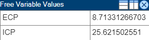
Free Variables Table

The Free Variable Values table displays the values of the optimization variables for the currently selected solution.

Range Constraint Output

The range constraint output is best explained using an example problem.

Description	Variables
Control parameters or free variables	S, EXH, INT
Fixed variables	N, L
Objective	Maximize TQ(S, EXH, INT, N, L) at the fixed values shown in this table. Run N L 1 3000 0.5 2 4000 0.6
Constraint	Restrict S between an upper and lower bound shown in this table. Run N L Min S Max S 1 3000 0.5 20 30 2 4000 0.6 30 40

When CAGE runs the optimization, the optimizer returns these optimal values of S, EXH and INT.

Run	N	L	Optimal S	Optimal EXH	Optimal INT
1	3000	0.5	21.33	8.593	29.839
2	4000	0.6	30	5	7.767

CAGE implements this range constraint: Lower Bound (LB) ≤ Expression ≤ Upper Bound (UB).

Specifically, CAGE implements these expressions.

Description	Expression
Two upper-bound constraints.	$$\left[\begin{array}{c}RangeConLeft(1)\\ RangeConLeft(2)\end{array}\right]=\left[\begin{array}{c}-Expression\\ Expression\end{array}\right]\le \left[\begin{array}{c}-LB\\ UB\end{array}\right]=\left[\begin{array}{c}RangeConRight(1)\\ RangeConRight(2)\end{array}\right]$$
Range constraint returns two values at each operating point within a run.	$$\left[\begin{array}{c}RangeConOut(1)\\ RangeConOut(2)\end{array}\right]=\left[\begin{array}{c}-Expression+LB\\ Expression-UB\end{array}\right]$$
Returned range constraints — Distance from the lower and upper bounds	RangeConOut(1) RangeConOut(2)
Constraint	LB(N,L) ≤ S ≤ UB(N,L)
CAGE implementation of constraint	$$\left[\begin{array}{c}-S\\ S\end{array}\right]\le \left[\begin{array}{c}-LB(N,L)\\ UB(N,L)\end{array}\right]$$
Two values at each operating point within a run to the optimizer	$$\left[\begin{array}{c}RangeConOut(1)\\ RangeConOut(2)\end{array}\right]=\left[\begin{array}{c}-S+LB(N,L)\\ S-UB(N,L)\end{array}\right]$$

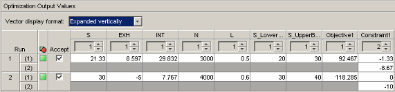
The Optimization Results pane shows the fixed variable settings, the optimal free variable settings, and the evaluation of objectives and constraints at the optimal free variable settings. In this example, the output of the range constraint at the optimal free variable settings is shown in the Constraint1 column. For each operating point in a run, two values are returned from the range constraint.

For the first run:

Description	Result
Optimal S value	21.33°
Distance from lower bound: RangeConOut(1)	–21.33°+20° = –1.33°
Distance from upper bound: RangeConOut(2)	21.33°–30° = –8.67°

Constraint Output

These are the values shown in the Constraint1 column. Remember that negative constraint values mean that the constraint is feasible. The same values appear in the Constraint Summary Table for the selected run, in the Constraint Value column, as shown in this figure.

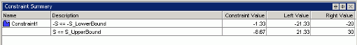
The Constraint Value gives a measure of the distance to the constraint boundary for each constraint output. If the Left Value > Right Value and greater than the tolerance for any of the constraint outputs, the constraint value is bold and the row is highlighted yellow. By default, CAGE takes this tolerance from the optimization constraint tolerance. You can control the value used for this highlighting by selecting View > Edit Constraint Tolerance. This means that this constraint distance should be checked to see if the constraint is feasible at that point.

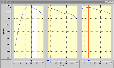
The Objective Graphs show cross-section plots of the objective function against each free variable in the problem. The left plot is a plot of the objective function against S, with EXH and INT at their optimal values, for the second run. The range constraint for the second operating point (30 ≤ S ≤ 40) is seen; the constraint region is white, and all other regions outside the constraint are yellow.

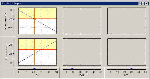
The constraint graphs for a range constraint shows how the Left Value of each output of a range constraint depends on the free variables in the optimization. The Left Value is compared with a plot of the Right Value output on the same axes. This comparison is illustrated for the example problem at the second run, as shown in the top left graph.

Constraint	Description
Constraint1(1)	First Left Value of the range constraint, RangeConLeft(1), for the first run in the example problem. The top-left graph shows a blue line, which is a plot of RangeConLeft(1) against S, with all other free variables set to their optimal values. The red horizontal line denotes the Right Value (RangeConRight(1), that is, the upper bound on S) which is -20°. Because this value is an upper bound, the yellow region above the red line shows where the table gradient constraint is infeasible. The vertical orange line shows the optimal value of S; the intersection of this line with the blue line is marked with a blue triangle on the Constraint1(1) axis—the triangle marks the Left Value (-21.3°) at the optimal settings. These are the Left and Right values in the Constraint Summary table for Constraint1(1).
Constraint1(2)	Second Left Value of the range constraint, RangeConLeft(2), for the first run in the example problem. The bottom left graph shows a blue line plot of RangeConLeft(2) against S, with all other free variables set to their optimal values. The horizontal red line denotes the Right Value (RangeConRight(2)), which is 30°. Because this value is an upper bound, the yellow region above the red line denotes where the table gradient constraint is infeasible. The vertical orange line shows the optimal value of S; the intersection of this with the blue line is marked with a blue triangle on the Constraint1(2) axis—the triangle marks the Left Value (21.3°) at the optimal settings. These are the Left and Right values in the Constraint Summary table for Constraint1(2).