正弦波から矩形波へ
この例では、矩形波に対するフーリエ級数展開が奇数個の高調波の和から構成されることを説明します。
まず、0 から 10 までの時間ベクトルを 0.1 刻みで作り、すべての点の正弦を求めます。この基本周波数をプロットします。
t = 0:.1:10;
y = sin(t);
plot(t,y);

次に、第 3 高調波を基本波に加えてプロットします。
y = sin(t) + sin(3*t)/3;
plot(t,y);
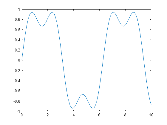
第 1、第 3、第 5、第 7、第 9 高調波を使います。
y = sin(t) + sin(3*t)/3 + sin(5*t)/5 + sin(7*t)/7 + sin(9*t)/9;
plot(t,y);
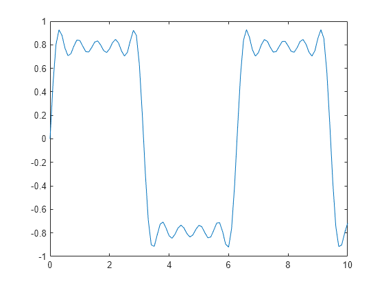
最後に、基本波から第 19 高調波までのすべてを順に使って、順次増えていく高調波のベクトルを作成し、すべての中間ステップを行列の行として保存します。
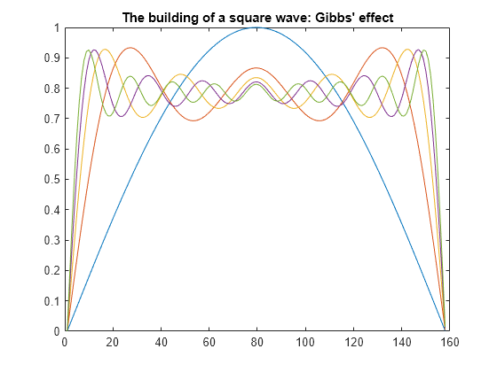
矩形波の形成過程を示すため、ベクトルを同じ Figure 上にプロットします。ギブス現象により、完全な矩形波になることはありません。
t = 0:.02:3.14;
y = zeros(10,length(t));
x = zeros(size(t));
for k = 1:2:19
   x = x + sin(k*t)/k;
   y((k+1)/2,:) = x;
end
plot(y(1:2:9,:)')
title('The building of a square wave: Gibbs'' effect')
正弦波から矩形波への段階的な変換を示す 3 次元の表面です。
surf(y);
shading interp
axis off ij
