Map Limit Properties
In many common situations, the map limit properties of
axesm-based maps, MapLatLimit and
MapLonLimit, provide a convenient way of specifying your map
projection origin or frame limits. Note that these properties are intentionally
redundant; you can always avoid them and instead use the Origin,
FLatLimit, and FLonLimit properties to set up
your map. When they're applicable, however, you'll probably find that it's easier and
more intuitive to set MapLatLimit and MapLonLimit,
especially when creating a new axesm-based map.
You typically use the MapLatLimit and
MapLonLimit properties to set up an
axesm-based map with a non-oblique, non-azimuthal projection, with
its origin on the Equator. (Most of the projections included in the Mapping Toolbox™ fall into this category; e.g., cylindrical, pseudo-cylindrical, conic, or
modified azimuthal.) In addition, even with a non-zero origin latitude (origin off the
Equator), you can use the MapLatLimit and
MapLonLimit properties with projections that are implemented
directly rather than via rotations of the sphere (e.g., tranmerc,
utm, lambertstd,
cassinistd, eqaconicstd,
eqdconicstd, and polyconicstd). This list
includes the projections used most frequently for large-scale maps, such as U.S.
Geological Survey topographic quadrangle maps. Finally, when the origin is located at a
pole or on the Equator, you can use the map limit properties with any azimuthal
projection (e.g., stereo, ortho,
breusing, eqaazim, eqdazim,
gnomonic, or vperspec).
On the other hand, you should avoid the map limit properties, working instead with the
Origin, FLatLimit, and
FLonLimit properties, when:
You want your map frame to be positioned asymmetrically with respect to the origin longitude.
You want to use an oblique aspect (that is, assign a non-zero rotation angle to the third element of the "orientation vector" supplied as the
Originproperty value).You want to change your projection's default aspect (normal vs. transverse).
You want to use a nonzero origin latitude, except in one of the special cases noted above.
You are using one of the following projections:
globe— No need for map limits; always covers entire planetcassini— Always in a transverse aspectwetch— Always in a transverse aspectbries— Always in an oblique aspect
There's no need to supply a value for the MapLatLimit property if
you've already supplied one for the Origin and
FLatLimit properties. In fact, if you supply all three when
calling either axesm or setm, the
FLatLimit value will be ignored. Likewise, if you supply values
for Origin, FLonLimit, and
MapLonLimit, the FLonLimit value will be
ignored.
If you do supply a value for either MapLatLimit or
MapLonLimit in one of the situations listed above,
axesm or setm will ignore it and issue a
warning. For example,
axesm('lambert','Origin',[40 0],'MapLatLimit',[20 70])
generates the warning message:
Ignoring value of MapLatLimit due to use of nonzero origin
 latitude with the lambert projection.
It's important to understand that MapLatLimit and
MapLonLimit are extra, redundant properties that are coupled to
the Origin, FLatLimit, and
FLonLimit properties. On the other hand, it's not too difficult
to know how to update your axesm-based map if you keep in mind the
following:
The
Originproperty takes precedence. It is set (implicitly, if not explicitly) every time you callaxesmand you cannot change it just by changing the map limits. (Note that when creating a newaxesm-based map, the map limits are used to help set the origin if it is not explicitly specified.)MapLatLimittakes precedence overFLatLimitif both are provided in the same call toaxesmorsetm, but changing either one alone affects the other.MapLonLimitandFLonLimithave a similar relationship.
The precedence of Origin means that if you want to reset your map
limits with setm and have setm also determine a
new origin, you must set Origin to [] in the same call. For
example,
setm(gca,'Origin',[],'MapLatLimit',newMapLatlim,...
   'MapLonLimit',newMapLonlim)
On the other hand, a call like this will automatically update the values of
FLatLimit and FLonLimit. Similarly, a call
like:
setm(gca,'FLatLimit',newFrameLatlim,'FLonLimit',newFrameLonlim)
will update the values of MapLatLimit and
MapLonLimit.
Finally, you probably don't want to try the following:
setm(gca,'Origin',[],'FLonLimit',newFrameLonlim)
because the value of FLonLimit (unlike
MapLonLimit) will not affect Origin, which
will merely change to a projection-dependent default value (typically [0 0
0]).
Specify Map Projection Origin and Frame Limits Automatically
This example shows how to specify the map projection origin and frame limits of axesm-based maps using the two map limit properties: MapLatLimit and MapLonLimit. While axesm-based maps support properties to set these values directly, Origin, FLatLimit, and FLonLimit, it is easier and more intuitive to use the map limit properties, especially when creating a new axesm-based map. This example highlights the interdependency of the axesm-based map limits and the map limit properties.
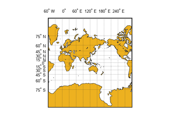
Create a map using a cylindrical projection or pseudo-cylindrical projection showing all or most of the Earth, with the Equator running as a straight horizontal line across the center of the map. The map is bounded by a geographic quadrangle and the projection origin is located on the Equator, centered between the longitude limits you specify using the map projection limits.
latlim = [-80 80];
lonlim = [100 -120];
figure
axesm('robinson','MapLatLimit',latlim,'MapLonLimit',lonlim,...
    'Frame','on','Grid','on','MeridianLabel','on','ParallelLabel','on')
axis off
setm(gca,'MLabelLocation',60)
load coastlines
plotm(coastlat,coastlon)
Check that the axesm function set the origin and frame limits based on the values you specified using the MapLatLim and MapLonLim properties. The longitude of the origin should be located halfway between the longitude limits of 100 E and 120 W. Since the map spans 140 degrees, adding half of 140 to the western limit, the origin longitude should be 170 degrees. The frame is centered on this longitude with a half-width of 70 degrees and the origin latitude is on the Equator.
origin = getm(gca,'Origin')origin = 1×3
0 170 0
flatlim = getm(gca,'FLatLimit')flatlim = 1×2
-80 80
flonlim = getm(gca,'FLonLimit')flonlim = 1×2
-70 70
Shift the western longitude to 40 degrees E (rather than 100 degrees) to include a little more of Asia. Use the setm function to assign a new value to the MapLonLimit property. Note the asymmetric appearance of the map.
setm(gca,'MapLonLimit',[40 -120])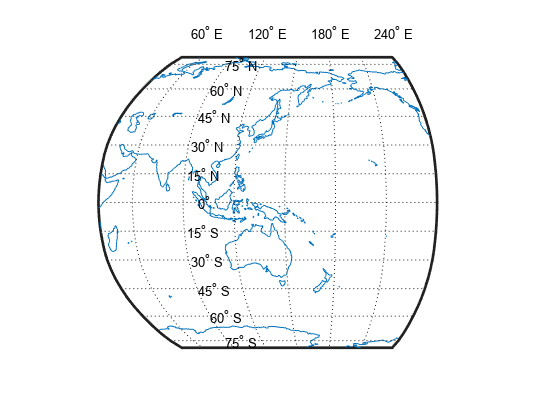
To correct the asymmetry, shift the western longitude again, this time specifying the origin. While the MapLatLimit and MapLonLimit properties are convenient, the values of the Origin, FLatLimit, and FLonLimit properties take precedence. You must specify the value of the origin to achieve the map you intended. The best way to do this is to specify an empty value for the Origin property and let the setm command calculate the value.
setm(gca,'MapLonLimit',[40 -120],'Origin',[])
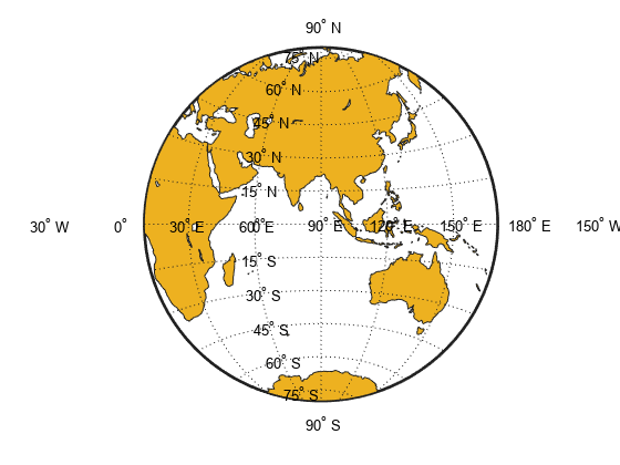
Create Cylindrical Projection Using Map Limit Properties
This example shows how to create cylindrical projection using map limit properties.
Load the coastline data.
load coastlinesConstruct a Mercator projection covering the full range of permissible latitudes with longitudes covering a full 360 degrees starting at 60 West.
figure('Color','w')
axesm('mercator','MapLatLimit',[-90 90],'MapLonLimit',[-60 300])
axis off;
framem on;
gridm on;
mlabel on;
plabel on;
setm(gca,'MLabelLocation',60)
geoshow(coastlat,coastlon,'DisplayType','polygon')
The previous call to axesm is equivalent to:
axesm('mercator','Origin',[0 120 0],'FlatLimit',[-90 90],'FLonLimit',[-180 180]);
You can verify this by checking the properties.
getm(gca,'Origin')ans = 1×3
0 120 0
getm(gca,'FLatLimit')ans = 1×2
-86 86
getm(gca,'FLonLimit')ans = 1×2
-180 180
Note that the map and frame limits are clamped to the range of [-86 86] imposed by the read-only TrimLat property.
getm(gca,'MapLatLimit')ans = 1×2
-86 86
getm(gca,'FLatLimit')ans = 1×2
-86 86
getm(gca,'TrimLat')ans = 1×2
-86 86
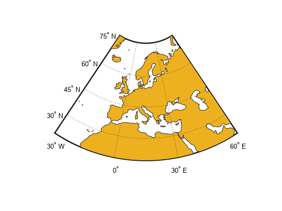
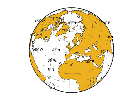
Create Conic Projection Using Map Limit Properties
This example shows how to create a map of the standard version of the Lambert Conformal Conic projection covering latitudes 20 North to 75 North and longitudes covering 90 degrees starting at 30 degrees West.
Load coastline data and display it. The call to axesm above is equivalent to: axesm('lambertstd','Origin', [0 15 0], 'FLatLimit',[20 75],FLonLimit',[-45 45])
load coastlines
figure('Color','w')
axesm('lambertstd','MapLatLimit',[20 75],'MapLonLimit',[-30 60])
axis off;
framem on;
gridm on;
mlabel on;
plabel on;
geoshow(coastlat, coastlon, 'DisplayType', 'polygon')
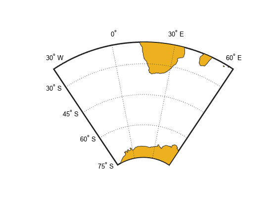
Create Southern Hemisphere Conic Projection
This example shows how to create a map of the standard version of the Lambert Conformal Conic projection into the Southern Hemisphere. The example overrides the default standard parallels and sets the MapLatLimit and MapLonLimit properties.
Load the coastline data MAT file, coastlines.mat.
load coastlinesDisplay the map, setting the MapLatLimit and MapLonLimit properties.
figure('Color','w')
axesm('lambertstd','MapParallels',[-75 -15], ...
		'MapLatLimit',[-75 -20],'MapLonLimit',[-30 60])
axis off
framem on
gridm on
mlabel on
plabel on
geoshow(coastlat,coastlon,'DisplayType','polygon')
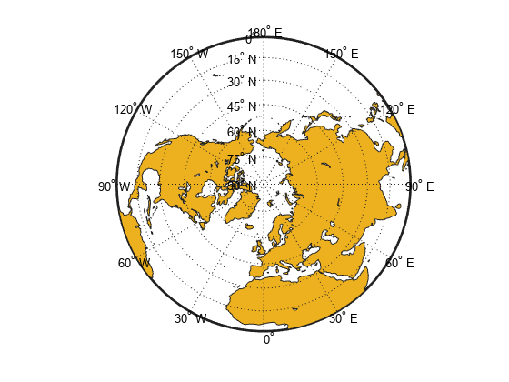
Create North-Polar Azimuthal Projection
This example shows how to construct a North-polar Equal-Area Azimuthal projection map extending from the Equator to the pole and centered by default on longitude 0.
Load coastline data set MAT file, coastlines.mat.
load coastlinesCreate map. The call to axesm is equivalent to: axesm('eqaazim','MLabelParallel',0,'Origin',[90 0 0],'FLatLimit',[-Inf 90]);
figure('Color','w')
axesm('eqaazim','MapLatLimit',[0 90])
axis off
framem on
gridm on
mlabel on
plabel on;
setm(gca,'MLabelParallel',0)
Plot the coast lines.
geoshow(coastlat,coastlon,'DisplayType','polygon')
Create South-Polar Azimuthal Projection
This example shows how to create a South-polar Stereographic Azimuthal projection map extending from the South Pole to 20 degrees S, centered on longitude 150 degrees West. Include a value for the Origin property in order to control the central meridian.
Load coastline data and display map.
load coastlines
figure('Color','w')
axesm('stereo','Origin',[-90 -150],'MapLatLimit',[-90 -20])
axis off;
framem on;
gridm on;
mlabel on;
plabel on;
setm(gca,'MLabelParallel',-20)
geoshow(coastlat,coastlon,'DisplayType','polygon')

The call to the axesm function above is equivalent to:
axesm('stereo','Origin',[-90 -150 0],'FLatLimit',[-Inf 70])
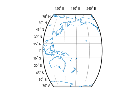
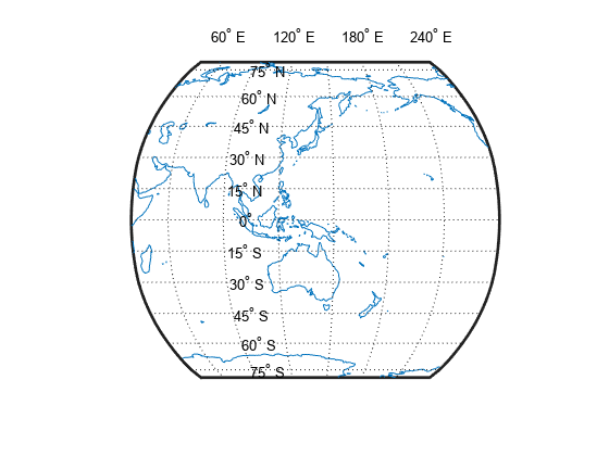
Create Equatorial Azimuthal Projection
This example shows how to create a map of an Equidistant Azimuthal projection with the origin on the Equator, covering from 10° E to 170° E. The origin longitude falls at the center of this range (90 E), and the map reaches north and south to within 10° of each pole.
Read coast data and display. The call to axesm is equivalent to axesm('eqaazim','Origin',[0 90 0],'FLatLimit',[-Inf 80]).
load coastlines
figure('Color','w')
axesm('eqdazim','FLatLimit',[],'MapLonLimit',[10 170])
axis off;
framem on;
gridm on;
mlabel on;
plabel on;
setm(gca,'MLabelParallel',0,'PLabelMeridian',60)
geoshow(coastlat,coastlon,'DisplayType','polygon')
Create General Azimuthal Projection
This example shows how to construct an Orthographic projection map with the origin centered near Paris, France. You can't use MapLatLimit or MapLonLimit here.
Read in coast data and display.
load coastlines
originLat = dm2degrees([48 48]);
originLon = dm2degrees([ 2 20]);

figure('Color','w')
axesm('ortho','Origin',[originLat originLon])
axis off; framem on; gridm on; mlabel on; plabel on;
setm(gca,'MLabelParallel',30,'PLabelMeridian',-30)
geoshow(coastlat,coastlon,'DisplayType','polygon')
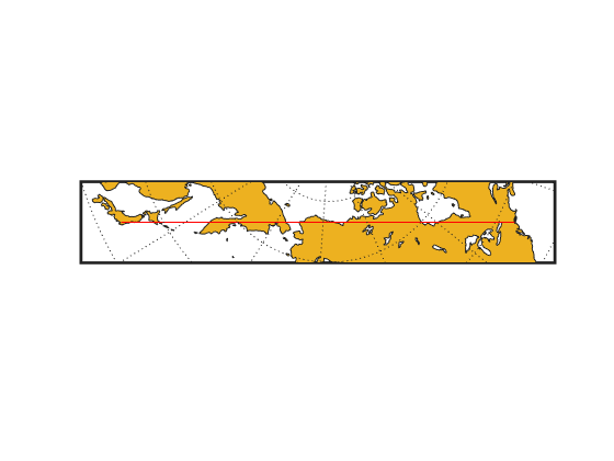
Create Long Narrow Oblique Mercator Projection
This example shows how to create a map with a long, narrow, oblique Mercator projection. The example shows the area 10 degrees to either side of the great-circle flight path from Tokyo to New York. You can't use MapLatLimit or MapLonLimit.
load coastlines
latTokyo = dm2degrees([ 35 40]);
lonTokyo = dm2degrees([139 45]);

latNewYork = dm2degrees([ 40 47]);
lonNewYork = dm2degrees([-73 58]);

[dist,az] = distance(latTokyo,lonTokyo,latNewYork,lonNewYork);
[midLat,midLon] = reckon(latTokyo,lonTokyo,dist/2,az);
midAz = azimuth(midLat,midLon,latNewYork,lonNewYork);

buf = [-10 10];

figure('Color','w')
axesm('mercator','Origin',[midLat midLon 90-midAz], ...
    'FLatLimit',buf,'FLonLimit',[-dist/2 dist/2] + buf)
axis off; framem on; gridm on; tightmap
geoshow(coastlat,coastlon,'DisplayType','polygon')
plotm([latTokyo latNewYork],[lonTokyo lonNewYork],'r-')