imdiffusefilt

Anisotropic diffusion filtering of images

Syntax

J = imdiffusefilt(I)

J = imdiffusefilt(I,Name=Value)

Description

J = imdiffusefilt(I) applies anisotropic diffusion filtering to image I and returns the result in J.

J = imdiffusefilt(I,Name=Value) uses name-value arguments to change the behavior of the anisotropic diffusion algorithm.

Examples

Perform Edge-Preserving Smoothing Using Anisotropic Diffusion

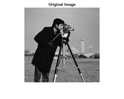
Read an image into the workspace and display it.

I = imread('cameraman.tif');
imshow(I)
title('Original Image')

Smooth the image using anisotropic diffusion. For comparison, also smooth the image using Gaussian blurring. Adjust the standard deviation sigma of the Gaussian smoothing kernel so that textured regions, such as the grass, are smoothed a similar amount for both methods.

Idiffusion = imdiffusefilt(I);
sigma = 1.2;
Igaussian = imgaussfilt(I,sigma);

Display the results.

montage({Idiffusion,Igaussian},'ThumbnailSize',[])
title('Smoothing Using Anisotropic Diffusion (Left) vs. Gaussian Blurring (Right)')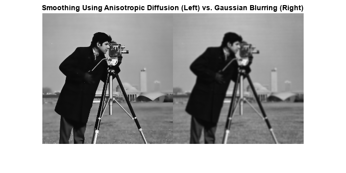

Anisotropic diffusion preserves the sharpness of edges better than Gaussian blurring.

Perform Edge-Aware Noise Reduction Using Anisotropic Diffusion

Read a grayscale image, then apply strong Gaussian noise to it. Display the noisy image.

I = imread('pout.tif');
noisyImage = imnoise(I,'gaussian',0,0.005);
imshow(noisyImage)
title('Noisy Image')

Compute the structural similarity index (SSIM) to measure the quality of the noisy image. The closer the SSIM value is to 1, the better the image agrees with the noiseless reference image.

n = ssim(I,noisyImage);
disp(['The SSIM value of the noisy image is ',num2str(n),'.'])

The SSIM value of the noisy image is 0.26556.

Reduce the noise using anisotropic diffusion. First, try the default parameters for the anisotropic diffusion filter, and display the result.

B = imdiffusefilt(noisyImage);
imshow(B)
title('Anisotropic Diffusion with Default Parameters')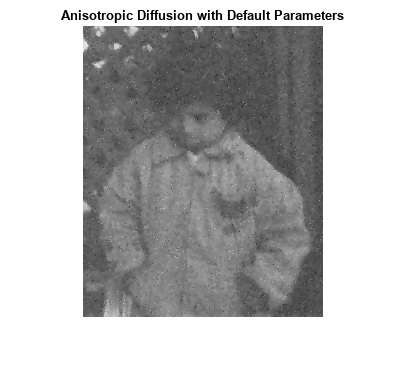

nB = ssim(I,B);
disp(['The SSIM value using default anisotropic diffusion is ',num2str(nB),'.'])

The SSIM value using default anisotropic diffusion is 0.65665.

The image is still degraded by noise, so refine the filter. Choose the quadratic conduction method because the image is characterized more by wide homogenous regions than by high-contrast edges. Estimate the optimal gradient threshold and number of iterations by using the imdiffuseest function. Display the resulting image.

[gradThresh,numIter] = imdiffuseest(noisyImage,'ConductionMethod','quadratic');
C = imdiffusefilt(noisyImage,'ConductionMethod','quadratic', ...
    'GradientThreshold',gradThresh,'NumberOfIterations',numIter);
imshow(C)
title('Anisotropic Diffusion with Estimated Parameters')

nC = ssim(I,C);
disp(['The SSIM value using quadratic anisotropic diffusion is ',num2str(nC),'.'])

The SSIM value using quadratic anisotropic diffusion is 0.88135.

Noise is less apparent in the resulting image. The SSIM value, which is closer to 1, confirms that the quality of the image has improved.

Perform 3-D Edge-Aware Noise Reduction

Load a noisy 3-D grayscale MRI volume.

load mristack

Perform edge-aware noise reduction on the volume using anisotropic diffusion. To prevent over-smoothing the low-contrast features in the brain, decrease the number of iterations from the default number, 5. The tradeoff is that less noise is removed.

diffusedImage = imdiffusefilt(mristack,'NumberOfIterations',3);

To compare the noisy image and the filtered image in detail, display the tenth slice of both.

imshowpair(mristack(:,:,10),diffusedImage(:,:,10),'montage')
title('Noisy Image (Left) vs. Anisotropic-Diffusion-Filtered Image (Right)')

Calculate the Naturalness Image Quality Evaluator (NIQE) score averaged over all slices in the volume. The NIQE score provides a quantitative measure of image quality that does not require a reference image. Lower NIQE scores reflect better perceptual image quality.

nframes = size(mristack,3);
m = 0;
d = 0;
for i = 1:nframes
    m = m + niqe(mristack(:,:,i));
    d = d + niqe(diffusedImage(:,:,i));
end
mAvg = m/nframes;
dAvg = d/nframes;
disp(['The NIQE score of the noisy volume is ',num2str(mAvg),'.'])

The NIQE score of the noisy volume is 5.7794.

disp(['The NIQE score using anisotropic diffusion is ',num2str(dAvg),'.'])

The NIQE score using anisotropic diffusion is 4.1391.

The NIQE score is consistent with the observation of reduced noise in the filtered image.

Input Arguments

I — Image to filter

2-D grayscale image | 3-D grayscale volume

Image to filter, specified as a 2-D grayscale image of size m-by-n or a 3-D grayscale volume of size m-by-n-by-k.

Note

To apply anisotropic diffusion filtering to a color image, use imdiffusefilt on each color channel independently.

Data Types: single | double | int8 | int16 | int32 | uint8 | uint16 | uint32

Name-Value Arguments

Specify optional pairs of arguments as Name1=Value1,...,NameN=ValueN, where Name is the argument name and Value is the corresponding value. Name-value arguments must appear after other arguments, but the order of the pairs does not matter.

Example: imdiffusefilt(I,NumberOfIterations=4,Connectivity="minimal") performs anisotropic diffusion on image I, using 4 iterations and minimal connectivity.

Before R2021a, use commas to separate each name and value, and enclose Name in quotes.

Example: imdiffusefilt(I,"NumberOfIterations",4,"Connectivity","minimal") performs anisotropic diffusion on image I, using 4 iterations and minimal connectivity.

GradientThreshold — Gradient threshold

numeric scalar | numeric vector

Gradient threshold, specified as a numeric scalar or a numeric vector of length NumberOfIterations. The value of GradientThreshold controls the conduction process by classifying gradient values as an actual edge or as noise. Increasing the value of GradientThreshold smooths the image more. The default value is 10% of the dynamic range of the image. You can use the imdiffuseest function to estimate a suitable value of GradientThreshold.

NumberOfIterations — Number of iterations

5 (default) | positive integer

Number of iterations to use in the diffusion process, specified as a positive integer. You can use the imdiffuseest function to estimate a suitable value of NumberOfIterations.

Connectivity — Connectivity

"maximal" (default) | "minimal"

Connectivity of a pixel to its neighbors, specified as one of these values:

• "maximal" — Considers 8 nearest neighbors for 2-D images, and 26 nearest neighbors for 3-D images

• "minimal" — Considers 4 nearest neighbors for 2-D images, and 6 nearest neighbors for 3-D images

ConductionMethod — Conduction method

"exponential" (default) | "quadratic"

Conduction method, specified as "exponential" or "quadratic". Exponential diffusion favors high-contrast edges over low-contrast edges. Quadratic diffusion favors wide regions over smaller regions.

Output Arguments

J — Diffusion-filtered image

numeric array

Diffusion-filtered image, returned as a numeric array of the same size and data type as the input image, I.

References

[1] Perona, P., and J. Malik. "Scale-space and edge detection using anisotropic diffusion." IEEE^® Transactions on Pattern Analysis and Machine Intelligence. Vol. 12, No. 7, July 1990, pp. 629–639.

[2] Gerig, G., O. Kubler, R. Kikinis, and F. A. Jolesz. "Nonlinear anisotropic filtering of MRI data." IEEE Transactions on Medical Imaging. Vol. 11, No. 2, June 1992, pp. 221–232.

Extended Capabilities

Thread-Based Environment

Run code in the background using MATLAB® backgroundPool or accelerate code with Parallel Computing Toolbox™ ThreadPool.

This function fully supports thread-based environments. For more information, see Run MATLAB Functions in Thread-Based Environment.

Version History

Introduced in R2018a

R2022b: Support for thread-based environments

imdiffusefilt now supports thread-based environments.