このページの内容は最新ではありません。最新版の英語を参照するには、ここをクリックします。

ラドン変換を使用したラインの検出

この例では、ラドン変換を使用してイメージ内のラインを検出する方法を説明します。ラドン変換は、ハフ変換として知られている一般的なコンピューター ビジョン演算と密接に関連しています。関数 radon を使用して、直線を検出するために使われるハフ変換を実行できます。

イメージのラドン変換の計算

イメージをワークスペースに読み取ります。それをグレースケール イメージに変換します。

I = fitsread("solarspectra.fts");
I = rescale(I);

元のイメージを表示します。

figure
imshow(I)
title("Original Image")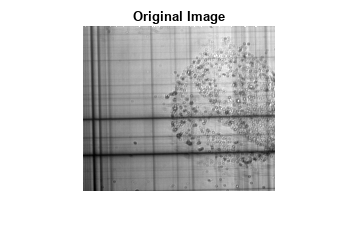

関数 edge を使用して、バイナリ エッジ イメージを計算します。関数 edge によって返されたバイナリ イメージを表示します。

BW = edge(I);
figure
imshow(BW)
title("Edges of Original Image")

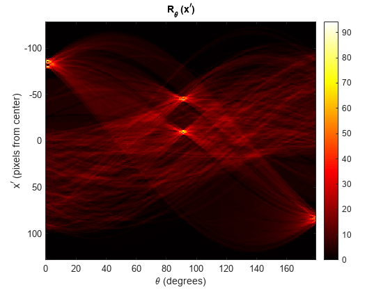
関数 radon を使用して、イメージのラドン変換を計算します。変換のピークの位置は、元のイメージ内の直線の位置に対応します。

theta = 0:179;
[R,xp] = radon(BW,theta);

ラドン変換の結果を表示します。

figure
imagesc(theta,xp,R)
colormap(hot)
xlabel("\theta (degrees)")
ylabel("x^{\prime} (pixels from center)")
title("R_{\theta} (x^{\prime})")
colorbar

ラドン変換のピークの解釈

5 つの最大ピークの "θ" および "x'" オフセット値を計算します。xp_peak_offset 値は、イメージの中心からのピークのオフセット (ピクセル単位) を表します。

R_sort = sort(unique(R),"descend");

[row_peak,col_peak] = find(ismember(R,R_sort(1:5)));
xp_peak_offset = xp(row_peak);
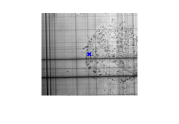
theta_peak = theta(col_peak);

元のイメージの中心に "x" マーカーを追加します。イメージの行インデックスは "y" 方向にマッピングされ、列インデックスは "x" 方向にマッピングされるため、centerX はイメージ I の列数の半分、centerY は行数の半分として計算します。

centerX = ceil(size(I,2)/2);
centerY = ceil(size(I,1)/2);

figure
imshow(I)
hold on
scatter(centerX,centerY,50,"bx",LineWidth=2)

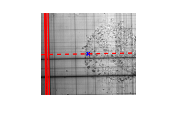
"θ" = 1 度、オフセットが中心から –80、–84、および –87 ピクセルのところに 3 つの強いピークが存在します。角度 "θ" = 1 度で中心を通る半径方向の直線を赤い破線としてプロットします。ラドンを、破線に垂直で中心から –80、–84、および –87 ピクセル シフトした赤い実線として表します。これにより、各実線が左側に配置されます。

[x1,y1] = pol2cart(deg2rad(1),5000);
plot([centerX-x1 centerX+x1],[centerY+y1 centerY-y1],"r--",LineWidth=2)

[x91,y91] = pol2cart(deg2rad(91),100);
for i=1:3
    plot([centerX-x91+xp_peak_offset(i) centerX+x91+xp_peak_offset(i)], ...
        [centerY+y91 centerY-y91], ...
        "r",LineWidth=2)
end

また、"θ" = 91 度、オフセットが中心から –8 および –44 ピクセルにも 2 つの強いピークが存在します。角度 "θ" = 91 度で中心を通る半径方向の直線を緑の破線としてプロットします。ラドン ピークを、破線に垂直で中心から –8 および –44 ピクセル シフトした緑の実線として表します。これにより、各実線が下側に配置されます。

plot([centerX-x91 centerX+x91],[centerY+y91 centerY-y91],"g--",LineWidth=2)

for i=4:5
plot([centerX-x1 centerX+x1], ...
    [centerY+y1-xp_peak_offset(i) centerY-y1-xp_peak_offset(i)], ...
    "g",LineWidth=2)
end

参考

radon | edge | pol2cart

関連するトピック

• ラドン変換