Create Human Eye Model Schematic
R2026bThis example shows how to construct an optical model of the human eye surface-by-surface. The model uses published parameters from the Navarro schematic eye [1] to define aspheric corneal surfaces, a crystalline lens, and a curved retinal surface.
Define Optical Media
The human eye contains four optically distinct media:
Corneal stroma
Aqueous humor
Crystalline lens
Vitreous humor
Specify the refractive index and Abbe number for each medium using the values in Tables 1 and 3 of [1]. The Abbe number quantifies chromatic dispersion, with lower values producing more dispersion.
nCornea = 1.376;
vCornea = 56.5;
nAqueous = 1.3374;
vAqueous = 49.61;
nLens = 1.42;
vLens = 48.0;
nVitreous = 1.336;
vVitreous = 50.9;
Create Optical System and Cornea
Create an opticalSystem object to represent the eye, then add the corneal surfaces. The cornea is the primary refracting element of the eye, contributing roughly 70% of the total optical power.
eye = opticalSystem(Name="Human Eye (Navarro 1985)");Add the cornea anterior surface, which forms the boundary between air and the eye surface, by using the addRefractiveSurface function. Specify a conic constant and radius of curvature to model the aspheric corneal shape. Specify the semi-diameter value as 6 millimeters [2].
addRefractiveSurface(eye, ...
    Radius=7.72,ConicConstant=-0.26, ...
    Material=[nCornea vCornea],SemiDiameter=6, ...
    DistanceToNext=0.55,Name="Cornea Anterior")
Add the cornea posterior surface, which forms the boundary between the cornea and aqueous humor. The aqueous thickness is 3.05 mm, and the iris sits 0.6 mm anterior to the lens.
addRefractiveSurface(eye, ...
    Radius=6.5,ConicConstant=0, ...
    Material=[nAqueous vAqueous],SemiDiameter=6, ...
    DistanceToNext=3.05-0.6,Name="Cornea Posterior")
Add Iris Diaphragm Inside Aqueous Humor
The iris sits inside the aqueous humor, approximately 0.6 mm anterior to the crystalline lens, according to the Gullstrand schematic eye model. To place an aperture stop inside a continuous medium, close the current lens element with a flat surface, insert the diaphragm, then open a new lens element carrying the same material. This three-step pattern prevents spurious optical power.
Close the aqueous element with a flat surface, which is a surface with an infinite radius.
addRefractiveSurface(eye, ...
    Radius=Inf,SemiDiameter=6,DistanceToNext=0)
Insert the iris diaphragm by using the addDiaphragm function. To model a pupil with a 3 mm radius, specify the SemiDiameter name-value argument as 1.5.
addDiaphragm(eye,SemiDiameter=1.5,DistanceToNext=0,Name="Iris")Continue the aqueous medium by opening a new element for the remaining 0.6 mm gap to the lens.
addRefractiveSurface(eye, ...
    Radius=Inf,Material=[nAqueous vAqueous], ...
    SemiDiameter=6,DistanceToNext=0.6)
Add Crystalline Lens
Add the crystalline lens, a biconvex element with strongly aspheric surfaces. The anterior surface introduces the lens material, and the posterior surface transitions to the vitreous humor.
addRefractiveSurface(eye, ...
    Radius=10.2,ConicConstant=-3.1316, ...
    Material=[nLens vLens],SemiDiameter=4.9, ...
    DistanceToNext=4,Name="Lens Anterior")
addRefractiveSurface(eye, ...
    Radius=-6,ConicConstant=-1, ...
    Material=[nVitreous vVitreous],SemiDiameter=4.9, ...
    DistanceToNext=16.4,Name="Lens Posterior")
Add Curved Retina and Image Plane
Create a curved retinal surface with a vitreous material on both sides by using the addRefractiveSurface function. The retina is a biconic surface, but image planes must be planar. Specifying the same vitreous material on both sides prevents refraction while preserving the curved geometry for ray intercepts.
Specify the Radius and ConicConstant name-value arguments using the biconic radii and conic constants, respectively, from Table 1 in [3].
retinaSD = 10.88;
addRefractiveSurface(eye, ...
    Radius=[-1000/77.37 -1000/80.57],ConicConstant=[0.30 0.25], ...
    Material=[nVitreous vVitreous], ...
    SemiDiameter=retinaSD,DistanceToNext=eps,Name="Retina")
addRefractiveSurface(eye, ...
    Radius=Inf,SemiDiameter=retinaSD,DistanceToNext=0, ...
    Name="Vitreous End")
Terminate the system with a flat image plane by using addImagePlane function.
addImagePlane(eye,SemiDiameter=retinaSD,Name="Image Plane")Visualize the Eye and Trace Rays
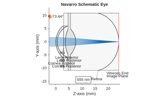
To verify the construction, display the system as a 2-D cross-section by using the view2d function, trace an on-axis ray bundle at 555 nm by using the traceRays function, and display the rays by using the addRays function. The wavelength 555 nm is the peak photopic sensitivity wavelength.
hv = view2d(eye,Title="Navarro Schematic Eye",Labels="surface")
hv =
  OpticalSystemViewer2D with properties:

            Title: "Navarro Schematic Eye"
    OpticalSystem: [1×1 opticalSystem]
           Labels: "surface"
      FieldPoints: "on"
             Rays: [0×0 optics.ui.Rays2D]
           Parent: [1×1 Figure]

  Show all properties
rb = traceRays(eye,Wavelengths=555);
addRays(hv,rb)
Inspect Paraxial Properties
To characterize first-order behavior, compute paraxial quantities by using the paraxialInfo function. The focal length should be approximately 16–17 mm for a relaxed emmetropic eye. The entrance pupil is the image of the iris as seen through the cornea. It appears slightly larger and more anterior than the physical iris due to corneal magnification.
pinfo = paraxialInfo(eye,Wavelength=555);
disp("Focal Length:     " + pinfo.FocalLength + " mm")
Focal Length: 16.4867 mm
disp("F-Number: f/" + pinfo.FNumber)F-Number: f/4.9805
disp("Entrance Pupil:   " + 2*pinfo.EntrancePupilRadius + ...
    " mm diameter at z = " + pinfo.EntrancePupilPosition(3) + " mm")
Entrance Pupil: 3.3102 mm diameter at z = 2.4549 mm
Compute the On-Axis Spot Diagram
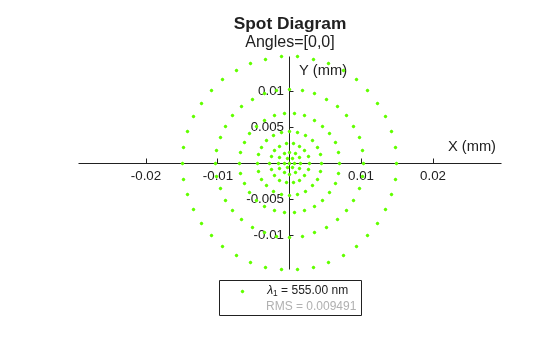
To evaluate image quality, compute the spot diagram at the image plane by using spot function. The on-axis spot is dominated by spherical aberration from the simplified model. For an on-axis field point, the spot function produces similar results on the flat image plane and the curved retinal surface.
result = spot(eye,Wavelengths=555);
show(result);
Extend the Model with Age and Accommodation Dependence
The static model represents a 25-year-old, relaxed eye. In reality, the crystalline lens changes significantly with age and accommodation, and refractive error shifts the retina relative to the focal point.
Age-dependent changes [4]:
Surface curvatures steepen — Anterior R decreases by –0.058 mm/year.
Lens thickness — Increases by +0.0236 mm/year.
Equivalent refractive index — Drops by –0.00039/year.
Accommodation-related changes [2],[5]:
Anterior curvature steepens, increasing power for near focus.
Lens thickness increases.
Refractive index increases slightly.
Maximum accommodation amplitude declines with age [6] by diopters.
Refractive error-related change:
Axial ametropia — Myopic eyes are longer and hyperopic eyes are shorter, shifting the retina relative to the focal point.
Use the HybridSchematicEye helper object to configure all of these dependencies together. Note that the model captures key optical behaviors, but does not fully replicate the real biological eye.
Measure Retinal Image Quality with Hybrid Schematic Eye Model
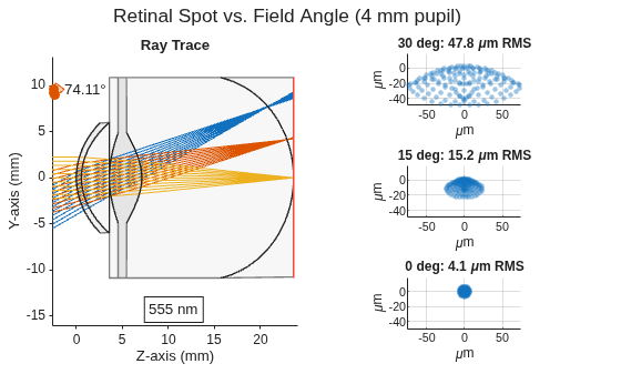
Use the HybridSchematicEye.retinalSpot function to trace rays to the curved retina surface and compute RMS spot size in the tangent plane at the chief ray. Each panel shows the retinal spot at increasing field angles.
hybridEye = HybridSchematicEye(Age=25,PupilDiameter=4);
angles = [30 0; 15 0; 0 0];
tiledlayout(height(angles),2,TileSpacing="compact",Padding="compact");
Trace rays through the eye model and display in the left column. Define the field points by using the fieldPoint function.
nexttile([height(angles) 1]);
fp = fieldPoint(Angle=angles);
rb = traceRays(hybridEye.OpticalSystem,FieldPoints=fp,Wavelengths=555);
hv = view2d(hybridEye.OpticalSystem,Title="Ray Trace")
hv =
OpticalSystemViewer2D with properties:
Title: "Ray Trace"
OpticalSystem: [1×1 opticalSystem]
Labels: "none"
FieldPoints: "on"
Rays: [0×0 optics.ui.Rays2D]
Parent: [1×1 TiledChartLayout]
Show all properties
addRays(hv,rb)
Compute and display the retinal spot at each field angle in the right column.
axHandles = gobjects(height(angles),1);
for k = 1:height(angles)
    axHandles(k) = nexttile;
    [rmsK,spots] = HybridSchematicEye.retinalSpot(hybridEye.OpticalSystem,FieldPoint=fieldPoint(Angle=[angles(k) 0]));
    scatter(spots(:,1)*1000,spots(:,2)*1000,12,"filled",MarkerFaceAlpha=0.4);
    axis equal
    grid on
    xlabel("\mum")
    ylabel("\mum")
    title(angles(k) + " deg: " + round(rmsK*1000,1) + " \mum RMS")
end
linkaxes(axHandles)
sgtitle("Retinal Spot vs. Field Angle (4 mm pupil)")
References
[1] Navarro, R., J. Santamaría, and J. Bescós. "Accommodation-Dependent Model of the Human Eye with Aspherics." Journal of the Optical Society of America A 2, no. 8 (1985): 1273–1281. https://doi.org/10.1364/JOSAA.2.001273.
[2] Schwiegerling, Jim. Field Guide to Visual and Ophthalmic Optics. SPIE Press, 2004.
[3] Atchison, David A., Nicola Pritchard, Katrina L. Schmid, Dion H. Scott, Catherine E. Jones, and James M. Pope. "Shape of the Retinal Surface in Emmetropia and Myopia." Investigative Ophthalmology & Visual Science 46, no. 8 (2005): 2698–2707. https://doi.org/10.1167/iovs.04-1506.
[4] Dubbelman, M., and G. L. Van der Heijde. "The Shape of the Aging Human Lens: Curvature, Equivalent Refractive Index and the Lens Paradox." Vision Research 41, no. 14 (2001): 1867–1877. https://doi.org/10.1016/S0042-6989(01)00057-8.
[5] Navarro, Rafael. "The Optical Design of the Human Eye: A Critical Review." Journal of Optometry 2, no. 1 (2009): 3–18. https://doi.org/10.3921/joptom.2009.3.
[6] Hofstetter, Henry W. "A Useful Age-Amplitude Formula." Optometric World 38 (1950): 42–45.

