動的システムの正則化による同定

R2026a

この例では、線形モデルと非線形モデルを同定するときに正則化を行う利点を説明します。

正則化とは

測定データを使用して動的システムを同定するときに、パラメーター推定値は以下のように決定されます。

$θ_{}^{ˆ} = a r g \min_{θ} V_{N} (θ)$

ここで、基準は通常、予測誤差 $ε (t, θ)$ の重み付き二次ノルムです。 $L_{2}$ の正則化された基準は次のように書き換えられます。

$θ_{}^{ˆ} = a r g \min_{θ} V_{N} (θ) + λ (θ - θ^{*})^{T} R (θ - θ^{*})$

この特殊例としてよく見られるのは、 $θ^{*} = 0, R = I$ の場合です。これは、統計学では "リッジ回帰" と呼ばれます。例は、Statistics and Machine Learning Toolbox™ の ridge コマンドを参照してください。

正則化については、 $θ^{*}$ が未知のパラメーターベクトルに関する事前情報を表し、 $λ * R$ がこの情報の信頼度を表す、と考えると役立ちます。( $λ * R$ が大きいほど信頼度が高くなります)。ベイズ理論の正式な解釈では、 $θ$ は、平均が $θ^{*}$ で共分散行列が $σ^{2} / λ R^{- 1}$ のガウス分布の "事前分布" をもちます。ここで、 $σ^{2}$ はイノベーションの分散です。

このため、正則化を使用するときには、システムに関するなんらかの事前情報を結び付けることができます。この情報は非常に不確実であることがあり、同様にシステムの安定性も不確実です。正則化変数 $λ$ および $R$ は、バイアスと分散とのトレードオフが最良となるような、優れたモデル複雑度を見つけるためのツールと見なすことができます。正則化定数 $λ$ および $R$ は、System Identification Toolbox™ のオプション Lambda および R によってそれぞれ表されます。 $θ^{*}$ の選択は、Nominal 正則化オプションによって制御されます。

FIR モデリングでのバイアスと分散のトレードオフ

線形システムのインパルス応答を FIR モデルとして推定する問題を考えます。

$y (t) = \sum_{k = 0}^{n b} g (k) u (t - k)$

これは、m = arx(z,[0 nb 0]) コマンドで推定されます。次数 nb の選択は、バイアス (誤差を大きくせずにゆっくり減衰するインパルス応答を捕捉するには nb を大きくする必要がある) と分散 (nb を大きくすると推定するパラメーターの個数が多くなり、分散が大きくなる) のトレードオフです。

これをシミュレーションの例で示します。システムとして 2 次バタワースフィルターを選択します。

$G (z) = \frac{0.02008 + 0.04017 z^{-} 1 + 0.02008 z^{-} 2}{1 - 1.561 z^{-} 1 + 0.6414 z^{-} 2}$

このインパルス応答を図 1 に示します。

trueSys = idtf([0.02008 0.04017 0.02008],[1 -1.561 0.6414],1);
[y0,t] = impulse(trueSys);
plot(t,y0)
xlabel('Time (seconds)'), ylabel('Amplitude'), title('Impulse Response')

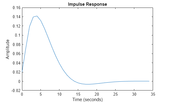
Figure contains an axes object. The axes object with title Impulse Response, xlabel Time (seconds), ylabel Amplitude contains an object of type line.

図 1: 真のインパルス応答

インパルス応答は 50 サンプル未満で 0 に減衰します。システムで生成したデータを使用して、これを推定します。ローパスフィルター処理したホワイトノイズを入力として使用してシステムをシミュレートし、分散 0.0025 をもつ微小のホワイトノイズの出力外乱を出力に加えます。1000 サンプルを収集します。このデータは regularizationExampleData.mat ファイルに保存され、図 2 に示されています。

load regularizationExampleData.mat eData
plot(eData)

MATLAB figure

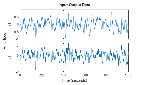
図 2: 推定に使用するデータ

優れた nb の値を決定するには、基本的にいくつかの値を使用して試行し、なんらかの検定手順でどれが最も優れているかを評価する必要があります。これは複数の方法で実行できますが、この例では真のシステムがわかっているので、nb=1,...,50 を指定してすべてのモデルをシミュレートし、真のインパルス応答を最もよく適合するモデルを見つけることで、理論的な最適値を決定することができます。このようなテストにより、nb = 13 でインパルス応答に対する最適な誤差ノルム (mse = 0.2522) が得られることが示されます。この推定インパルス応答と真のインパルス応答を図 3 に示します。

nb = 13;
m13 = arx(eData,[0 nb 0]);

[y13,~,~,y13sd] = impulse(m13,t);
plot(t,y0,t,y13)
xlabel('Time (seconds)'), ylabel('Amplitude'), title('Impulse Response')
legend('True system','13:th order FIR model')

Figure contains an axes object. The axes object with title Impulse Response, xlabel Time (seconds), ylabel Amplitude contains 2 objects of type line. These objects represent True system, 13:th order FIR model.

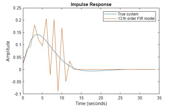
図 3: 真のインパルス応答と次数 nb = 13 の推定応答

非常に優れた信号対ノイズ比をもつデータ点 1000 点を使用しても、推定したインパルス応答の形状は大きく異なります。推定したインパルス応答の不確かさも非常に大きく、これは応答の標準偏差 1 の値で示されます。この理由は、ローパス入力の励起が弱いからです。

plot(t,y0,t,y13,t,y13+y13sd,'r:',t,y13-y13sd,'r:')
xlabel('Time (seconds)'), ylabel('Amplitude'), title('Impulse Response')
legend('True system','13:th order FIR model','Bounds')

Figure contains an axes object. The axes object with title Impulse Response, xlabel Time (seconds), ylabel Amplitude contains 4 objects of type line. These objects represent True system, 13:th order FIR model, Bounds.

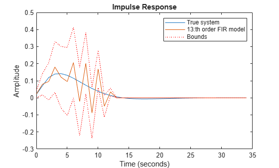
図 4: 標準偏差 1 に対応する信頼限界をもつ推定応答

このため、次数 50 の FIR モデルのリッジ回帰を使用して、良好なバイアスと分散のトレードオフを行います。arxOptions を使用して正則化定数を設定します。この演習では単純なペナルティ $| | θ | |^{2}$ を適用します。

aopt = arxOptions;
aopt.Regularization.Lambda = 1;
m50r = arx(eData, [0 50 0], aopt);

得られた推定応答と真のインパルス応答との誤差ノルムは 0.1171 であり、この結果を信頼限界と共に図 5 で示します。

[y50r,~,~,y50rsd] = impulse(m50r,t);
plot(t,y0,t,y50r,t,y50r+y50rsd,'r:',t,y50r-y50rsd,'r:')
xlabel('Time (seconds)'), ylabel('Amplitude'), title('Impulse Response')
legend('True system','50:th order regularized estimate')

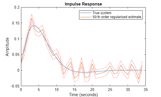
図 5: 真のインパルス応答とリッジ正則化した次数 nb = 50 の推定インパルス応答

明らかに、正則化を行わずに FIR の最適な次数を選択するよりも、単純に正則化を選択するほうが良好なバイアスと分散のトレードオフを得られます。

FIR モデルの正則化定数の自動決定

さらに優れた結果を得ることができます。真のインパルス応答は 0 に減衰しかつ滑らかな形状であるという見識を使用することで、 $R, λ$ の選択をデータに合わせてカスタマイズできます。これは、関数 arxRegul によって実行できます。

[L,R] = arxRegul(eData,[0 50 0],arxRegulOptions('RegularizationKernel','TC'));
aopt.Regularization.Lambda = L;
aopt.Regularization.R = R;
mrtc = arx(eData, [0 50 0], aopt);
[ytc,~,~,ytcsd] = impulse(mrtc,t);

arxRegul は Optimization Toolbox™ の fmincon を使用して、正則化カーネル (ここでは "TC") に関連付けられているハイパーパラメーターを計算します。Optimization Toolbox が使用できない場合は、代わりにガウス・ニュートン法による単純な検索スキームを使用します。arxRegulOptions の "Advanced.SearchMethod" オプションを使用して、検索方法を明示的に選択します。その後、推定されたハイパーパラメーターを使用して $R$ および $λ$ の値を導出します。

$R$ および $λ$ の推定値を ARX で使用することにより、誤差ノルム 0.0461 が得られます。その応答を図 6 に示します。このように調整した正則化は impulseest コマンドでも実行できます。図に示すように、正則化しない応答と比較して分散が大幅に小さくなり、インパルス応答の適合が良好になります。推定応答の分散が小さくなるとバイアスが大きくなりますが、この例でのバイアスの増加はほんのわずかです。

plot(t,y0,t,ytc,t,ytc+ytcsd,'r:',t,ytc-ytcsd,'r:')
xlabel('Time (seconds)'), ylabel('Amplitude'), title('Impulse Response')
legend('True system','50:th order tuned regularized estimate')

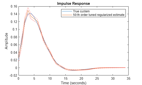
図 6: 真のインパルス応答と調整正則化した次数 nb = 50 の推定応答

正則化 ARX モデルによる状態空間モデルの推定

有色測定ノイズをもつ 30 次線形システムであるシステム m0 を考えます。

$y (t) = G (q) u (t) + H (q) e (t)$

G(q) は入力から出力への伝達関数、H(q) は外乱の伝達関数です。このシステムは、regularizationExampleData.mat データファイルに格納されています。G(q) と H(q) のインパルス応答を図 7 に示します。

load regularizationExampleData.mat m0
m0H = noise2meas(m0); % the extracted noise component of the model
[yG,t] = impulse(m0);
yH = impulse(m0H,t);

clf
subplot(211)
plot(t, yG)
title('Impulse Response of G(q)'), ylabel('Amplitude')

subplot(212)
plot(t, yH)
title('Impulse Response of H(q)'), ylabel('Amplitude')
xlabel('Time (seconds)')

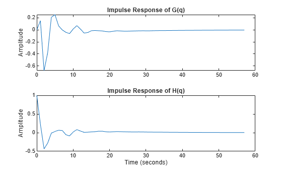
Figure contains 2 axes objects. Axes object 1 with title Impulse Response of G(q), ylabel Amplitude contains an object of type line. Axes object 2 with title Impulse Response of H(q), xlabel Time (seconds), ylabel Amplitude contains an object of type line.

図 7: G(q) のインパルス応答 (上) と H(q) のインパルス応答 (下)

分散 1 のホワイトノイズ入力 u と分散 0.1 のノイズレベル e を使用して m0 をシミュレートし、210 のデータ点を収集しました。このデータは regularizationExampleData.mat に格納されているもので、以下の図に示します。

load regularizationExampleData.mat m0simdata
clf
plot(m0simdata)

MATLAB figure

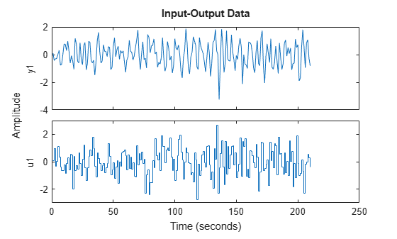
図 8: 推定に使用するデータ

これらのデータから m0 のインパルス応答を推定するために、イノベーション形式の状態空間モデル (または同等の ARMAX モデル) を使用し、前述の例と同様に impulse コマンドを使用してインパルス応答を計算することができます。状態空間モデルの計算には、以下のような構文を使用することができます。

mk = ssest(m0simdata, k, 'Ts', 1);

問題は、適切な次数 k を決定することです。一般的に使用されている方法が 2 つあります。

交差検定 (CV): データの前半 ze = m0simdata(1:150) を使用して k = 1,...,maxo の mk を推定し、compare コマンドを以下のように使用してデータの後半 zv = m0simdata(151:end) への適合を評価します。[~,fitk] = compare(zv, mk, compareOptions('InitialCondition', 'z'))。最もよい適合が得られる次数 k を決定します。データレコード全体を使用して、モデルを再度推定します。
赤池基準 (AIC) の使用: データセット全体を使用して次数 k = 1,...,maxo のモデルを推定し、次に aic(mk) を最小にするモデルを選択します。

最大次数 maxo = 30 を使用してこれらの手法をデータに適用すると、CV では k = 15、AIC では k = 3 が選択されます。

"理論的" テスト: CV と AIC のテストに加えて、G(q) (または H(q)) の真のインパルス応答に最もよく適合する推定モデルの次数 k を調べることもできます。これには当然、真のシステム m0 の情報が必要ですが、この情報を得ることは困難です。ただし、m0 が既知である例についてこの比較を実行した場合、k = 12 のときに推定モデルのインパルス応答が m0 (=|G(q)|) のインパルス応答に最もよく適合することがわかります。同様に、k = 3 のときに、推定モデルのノイズ成分のインパルス応答が m0 (=|H(q)|) のノイズ成分のインパルス応答に最もよく適合することがわかります。理論的テストは、さまざまな次数と正則化パラメーターを使用して生成したモデルの品質を比較する基準点を設定するものです。

さまざまな次数の選択基準について計算したインパルス応答を比較します。

m3 = ssest(m0simdata, 3, 'Ts', 1);
m12 = ssest(m0simdata, 12, 'Ts', 1);
m15 = ssest(m0simdata, 15, 'Ts', 1);

y3 = impulse(m3, t); 
y12 = impulse(m12, t);
y15 = impulse(m15, t);

plot(t,yG, t,y12, t,y15, t,y3)
xlabel('Time (seconds)'), ylabel('Amplitude'), title('Impulse Response')
legend('True G(q)',...
   sprintf('Oracle choice: %2.4g%%',100*(1-goodnessOfFit(y12,yG,'NRMSE'))),...
   sprintf('CV choice: %2.4g%%',100*(1-goodnessOfFit(y15,yG,'NRMSE'))),...
   sprintf('AIC choice: %2.4g%%',100*(1-goodnessOfFit(y3,yG,'NRMSE'))))

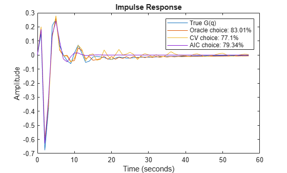
図 9: G(q) の真のインパルス応答とさまざまな次数をもつ推定モデルの比較

yH3 = impulse(noise2meas(m3), t); 
yH15 = impulse(noise2meas(m15), t);

plot(t,yH, t,yH3, t,yH15, t,yH3)
xlabel('Time (seconds)'), ylabel('Amplitude'), title('Impulse Response')
legend('True H(q)',...
   sprintf('Oracle choice: %2.4g%%',100*(1-goodnessOfFit(yH3,yH,'NRMSE'))),...
   sprintf('CV choice: %2.4g%%',100*(1-goodnessOfFit(yH15,yH,'NRMSE'))),...
   sprintf('AIC choice: %2.4g%%',100*(1-goodnessOfFit(yH3,yH,'NRMSE'))))

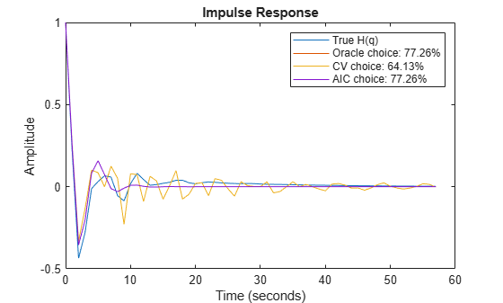
図 10: H(q) の真のインパルス応答とさまざまな次数をもつ推定ノイズモデルの比較

複数の状態空間モデルのうち、G(q) について 83% の優れた適合を得ることが可能であるとわかりましたが、次数の選択手順で最適な次数を見つけられないことがあります。

次に、正則化で何が得られるかを調べます。以下のコードを実行して、次数のかなり高い正則化した ARX モデルを推定します。

aopt = arxOptions;
[Lambda, R] = arxRegul(m0simdata, [5 60 0], arxRegulOptions('RegularizationKernel','TC'));
aopt.Regularization.R = R;
aopt.Regularization.Lambda = Lambda;
mr = arx(m0simdata, [5 60 0], aopt); 
nmr = noise2meas(mr);
ymr = impulse(mr, t); 
yHmr = impulse(nmr, t); 
fprintf('Goodness of fit for ARX model is: %2.4g%%n',100*(1-goodnessOfFit(ymr,yG,'NRMSE')))

Goodness of fit for ARX model is: 83.12%

fprintf('Goodness of fit for noise component of ARX model is: %2.4g%%n',100*(1-goodnessOfFit(yHmr,yH,'NRMSE')))

Goodness of fit for noise component of ARX model is: 78.71%

この正則化した ARX モデルは、理論的な選択よりもさらによく真の G(q) に適合していることがわかりました。H(q) の適合は 80 % を上回り、これは最適なノイズモデルを求める理論的な次数選択よりも優れています。mr が高次 (状態数 60) モデルであり、低次の状態空間モデルと比較することは不当であるという反論もあるでしょう。ただし、balred コマンド (Control System Toolbox™ が必要) を使用して、この高次モデルをたとえば 7 次に低次元化することができます。

mred7 = balred(idss(mr),7);
nmred7 = noise2meas(mred7);
y7mr = impulse(mred7, t); 
y7Hmr = impulse(nmred7, t);

図 11 と図 12 に、正則化と低次元化を行った正則化モデルと、正確性を損なうことなく状態空間次数を理論的に選択した ssest との比較を示します。

plot(t,yG, t,y12, t,ymr, t,y7mr)
xlabel('Time (seconds)'), ylabel('Amplitude'), title('Impulse Response')
legend('True G(q)',...
   sprintf('Oracle choice: %2.4g%%',100*(1-goodnessOfFit(y12,yG,'NRMSE'))),...
   sprintf('High order regularized: %2.4g%%',100*(1-goodnessOfFit(ymr,yG,'NRMSE'))),...
   sprintf('Reduced order: %2.4g%%',100*(1-goodnessOfFit(y7mr,yG,'NRMSE'))))

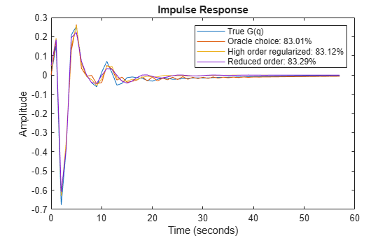
図 11: 正則化モデルと理論的に次数を選択した G(q) との比較

plot(t,yH, t,yH3, t,yHmr, t,y7Hmr)
xlabel('Time (seconds)'), ylabel('Amplitude'), title('Impulse Response')
legend('True H(q)',...
   sprintf('Oracle choice: %2.4g%%',100*(1-goodnessOfFit(yH3,yH,'NRMSE'))),...
   sprintf('High order regularized: %2.4g%%',100*(1-goodnessOfFit(yHmr,yH,'NRMSE'))),...
   sprintf('Reduced order: %2.4g%%',100*(1-goodnessOfFit(y7Hmr,yH,'NRMSE'))))

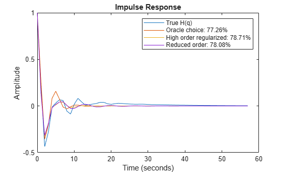
図 12: 正則化モデルと理論的に次数を選択した H(q) との比較

ARX モデルの次数の選択は、ssest での状態空間モデルの次数の選択と同様に影響を受けやすい決定かどうかという疑問をもつことは当然です。arx(z,[10 50 0], aopt) などを使用した単純なテストを実行すると、G(q) の適合の変化はわずかであることが示されます。

低次元化による正則化手法を使用した状態空間モデルの推定

高次 ARX モデルを推定した後、状態空間に変換して目的の次数へ低次元化する前述の手順は、ssregest コマンドを使用して自動化することができます。ssregest ではこの手順を大幅に簡略化できるのと同時に、直達値や遅延値の指定により最適な次数を求める、モデル構造を微調整するなどのその他の役立つオプションも利用できます。ここで ssregest を使用して、mred7 に類似する低次元化モデルを単純に再度推定します。

opt = ssregestOptions('ARXOrder',[5 60 0]); 
mred7_direct = ssregest(m0simdata, 7, 'Feedthrough', true, opt);
compare(m0simdata, mred7, mred7_direct)

MATLAB figure

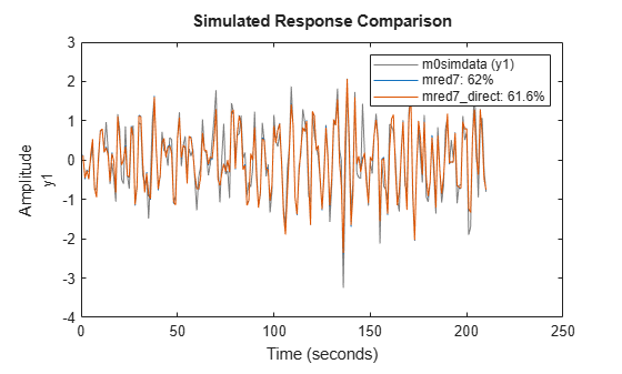
図 13: 推定データに対する状態空間モデルの応答の比較

h = impulseplot(mred7, mred7_direct, 40);
showConfidence(h,1) %  1 s.d. "zero interval"
hold on
s = stem(t,yG,'r');
s.DisplayName = 'True G(q)';
legend('show')

MATLAB figure

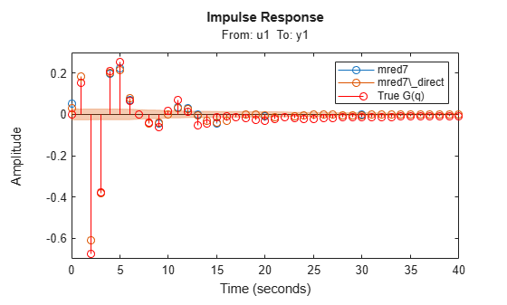
図 14: 状態空間モデルのインパルス応答の比較

図 14 の信頼限界は、モデル mred7_direct についてのみ表示されています。これは、モデル mred7 については信頼限界が計算されていないからです。同定されたモデルの任意の変換 (ここでは balred) について、translatecov コマンドを使用して信頼限界を生成できます。また、ssregest コマンドには "ARXOrder" オプションの値を指定する必要がありません。値を明示的に指定しない場合は、データ長に基づいて自動的に選択されます。

グレーボックスモデルの基本的なバイアスと分散のトレードオフ

ここでは、事前情報が観測データの情報と一致する代表的な場合のグレーボックス推定について説明します。これらの情報源の間でバランスがとれたトレードオフが得られることはよいことであり、正則化がそのための主要ツールになります。

角速度の静的ゲイン G と時定数 $τ$ をもつ DC モーターを考えます (iddemo7 などを参照)。

$G (s) = \frac{G}{s (1 + s τ)}$

状態空間形式で表すと、以下の式が得られます。

${x_{1}}_{}^{˙} = x_{2}$

${x_{2}}_{}^{˙} = - 1 / τ \cdot x_{2}$

$y = x + e$

ここで、 $x = [x_{1}; x_{2}]$ は状態ベクトルであり、角度 $x_{1}$ と速度 $x_{2}$ で構成されています。出力方程式に示されるように、両方の状態をノイズとして観測します。

事前情報と経験から、 $G$ は約 4、 $τ$ は約 1 であると考えます。motorData にシステムから大量のノイズを含むデータ 400 点を収集します。各成分の e の標準偏差は 50 です。また、比較の目的で、同じモデルのノイズを含まないシミュレーションデータも保存します。このデータを図 15 に示します。

load regularizationExampleData.mat motorData motorData_NoiseFree
t = motorData.SamplingInstants;
subplot(311)
plot(t,[motorData_NoiseFree.y(:,1),motorData.y(:,1)])
ylabel('Output 1')
subplot(312)
plot(t,[motorData_NoiseFree.y(:,2),motorData.y(:,2)])
ylabel('Output 2')
subplot(313)
plot(t,motorData_NoiseFree.u) % input is the same for both datasets
ylabel('Input')
xlabel('Time (seconds)')

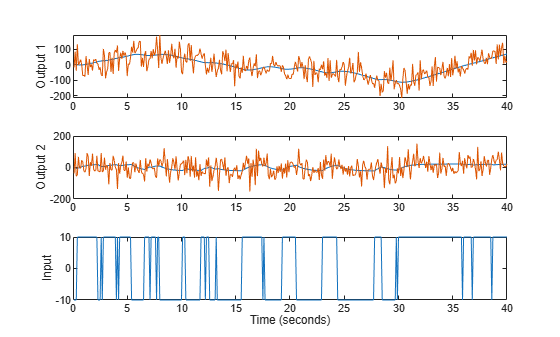
Figure contains 3 axes objects. Axes object 1 with ylabel Output 1 contains 2 objects of type line. Axes object 2 with ylabel Output 2 contains 2 objects of type line. Axes object 3 with xlabel Time (seconds), ylabel Input contains an object of type line.

図 15: 検定に使用するノイズのないシミュレーションデータに、グレーボックス推定に使用するノイズを含むデータを重ね合わせた図。上から順に、角度、角速度、入力電圧。

このシミュレーションの真のパラメーター値は G = 2.2、 $τ$ = 0.8 です。モデルを推定するために、idgrey モデルファイル DCMotorODE.m を作成します。

type('DCMotorODE')

function [A,B,C,D] = DCMotorODE(G,Tau,Ts)
%DCMOTORODE ODE file representing the dynamics of a DC motor parameterized
%by gain G and time constant Tau.
%
%   [A,B,C,D,K,X0] = DCMOTORODE(G,Tau,Ts) returns the state space matrices
%   of the DC-motor with time-constant Tau and static gain G. The sample
%   time is Ts.
%
%   This file returns continuous-time representation if input argument Ts
%   is zero. If Ts>0, a discrete-time representation is returned.
%
% See also IDGREY, GREYEST.

%   Copyright 2013 The MathWorks, Inc.

A = [0 1;0 -1/Tau];
B = [0; G/Tau];
C = eye(2);
D = [0;0];
if Ts>0 % Sample the model with sample time Ts
   s = expm([[A B]*Ts; zeros(1,3)]);
   A = s(1:2,1:2);
   B = s(1:2,3);
end

これにより、idgrey オブジェクトが以下のように作成されます。

mi = idgrey(@DCMotorODE,{'G', 4; 'Tau', 1},'cd',{}, 0);

ここで、予測したパラメーター値を初期値として挿入しています。greyest コマンドを使用して、観測データの情報に合わせてこのモデルを調整します。

m = greyest(motorData, mi)

m =
  Continuous-time linear grey box model defined by @DCMotorODE function:
      dx/dt = A x(t) + B u(t) + K e(t)
       y(t) = C x(t) + D u(t) + e(t)
 
  A = 
           x1      x2
   x1       0       1
   x2       0  -1.741
 
  B = 
          u1
   x1      0
   x2  3.721
 
  C = 
       x1  x2
   y1   1   0
   y2   0   1
 
  D = 
       u1
   y1   0
   y2   0
 
  K = 
       y1  y2
   x1   0   0
   x2   0   0
 
  Model parameters:
   G = 2.138
   Tau = 0.5745
 
Parameterization:
   ODE Function: @DCMotorODE
   (parametrizes both continuous- and discrete-time equations)
   Disturbance component: none
   Initial state: 'auto'
   Number of free coefficients: 2
   Use "getpvec", "getcov" for parameters and their uncertainties.

Status:                                                 
Estimated using GREYEST on time domain data "motorData".
Fit to estimation data: [29.46;4.167]%                  
FPE: 6.074e+06, MSE: 4908                               
 
Model Properties

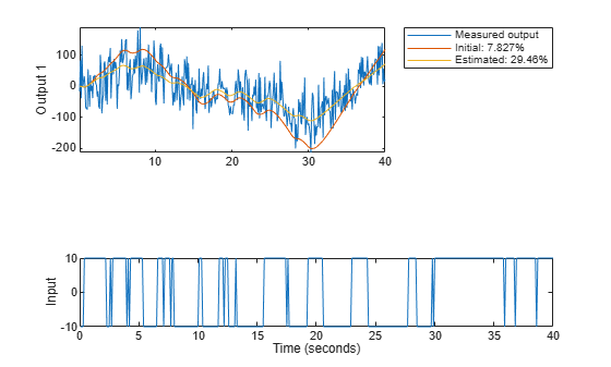
モデル m のパラメーターは $τ$ = 0.57、G = 2.14 であり、再現したデータを図 16 に示します。

copt = compareOptions('InitialCondition', 'z');
[ymi, fiti] = compare(motorData, mi, copt);
[ym, fit] = compare(motorData, m, copt);
t = motorData.SamplingInstants;
subplot(211)
plot(t, [motorData.y(:,1), ymi.y(:,1), ym.y(:,1)])
axis tight
ylabel('Output 1')
legend({'Measured output',...
   sprintf('Initial: %2.4g%%',fiti(1)),...
   sprintf('Estimated: %2.4g%%',fit(1))},...
   'Location','BestOutside')

Figure contains 2 axes objects. Axes object 1 with xlabel Time (seconds), ylabel Input contains an object of type line. Axes object 2 with ylabel Output 1 contains 3 objects of type line. These objects represent Measured output, Initial: 7.827%, Estimated: 29.46%.

subplot(212)
plot(t, [motorData.y(:,2), ymi.y(:,2), ym.y(:,2)])
ylabel('Output 2')
axis tight
legend({'Measured output',...
   sprintf('Initial: %2.4g%%',fiti(2)),...
   sprintf('Estimated: %2.4g%%',fit(2))},...
   'Location','BestOutside')

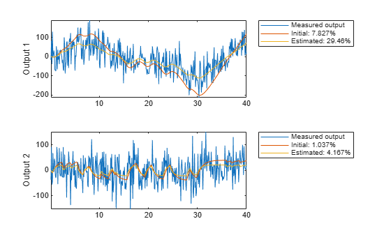
Figure contains 2 axes objects. Axes object 1 with ylabel Output 1 contains 3 objects of type line. These objects represent Measured output, Initial: 7.827%, Estimated: 29.46%. Axes object 2 with ylabel Output 2 contains 3 objects of type line. These objects represent Measured output, Initial: 1.037%, Estimated: 4.167%.

図 16: 測定出力および初期モデルと推定モデルのモデル出力

このシミュレーションの例では、ノイズのないデータ (motorData_NoiseFree) にもアクセスしているため、ノイズのないデータへの適合を図 17 に示します。

[ymi, fiti] = compare(motorData_NoiseFree, mi, copt);
[ym, fit] = compare(motorData_NoiseFree, m, copt);
subplot(211)
plot(t, [motorData_NoiseFree.y(:,1), ymi.y(:,1), ym.y(:,1)])
axis tight
ylabel('Output 1')
legend({'Noise-free output',...
   sprintf('Initial: %2.4g%%',fiti(1)),...
   sprintf('Estimated: %2.4g%%',fit(1))},...
   'Location','BestOutside')
subplot(212)
plot(t, [motorData_NoiseFree.y(:,2), ymi.y(:,2), ym.y(:,2)])
ylabel('Output 2')
axis tight
legend({'Noise-free output',...
   sprintf('Initial: %2.4g%%',fiti(2)),...
   sprintf('Estimated: %2.4g%%',fit(2))},...
   'Location','BestOutside')

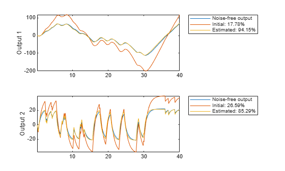
Figure contains 2 axes objects. Axes object 1 with ylabel Output 1 contains 3 objects of type line. These objects represent Noise-free output, Initial: 17.78%, Estimated: 94.15%. Axes object 2 with ylabel Output 2 contains 3 objects of type line. These objects represent Noise-free output, Initial: 26.59%, Estimated: 85.29%.

図 17: ノイズのない出力および初期モデルと推定モデルのモデル出力

パラメーターの推定値を見ると、ノイズを含むデータを使用した推定値が事前の物理情報と大きく異なることがわかります。データ情報を事前情報とマージするために、正則化を使用します。

opt = greyestOptions;
opt.Regularization.Lambda = 100;
opt.Regularization.R = [1, 1000]; % second parameter better known than first
opt.Regularization.Nominal = 'model';
mr = greyest(motorData, mi, opt)

mr =
  Continuous-time linear grey box model defined by @DCMotorODE function:
      dx/dt = A x(t) + B u(t) + K e(t)
       y(t) = C x(t) + D u(t) + e(t)
 
  A = 
           x1      x2
   x1       0       1
   x2       0  -1.119
 
  B = 
          u1
   x1      0
   x2  2.447
 
  C = 
       x1  x2
   y1   1   0
   y2   0   1
 
  D = 
       u1
   y1   0
   y2   0
 
  K = 
       y1  y2
   x1   0   0
   x2   0   0
 
  Model parameters:
   G = 2.187
   Tau = 0.8938
 
Parameterization:
   ODE Function: @DCMotorODE
   (parametrizes both continuous- and discrete-time equations)
   Disturbance component: none
   Initial state: 'auto'
   Number of free coefficients: 2
   Use "getpvec", "getcov" for parameters and their uncertainties.

Status:                                                 
Estimated using GREYEST on time domain data "motorData".
Fit to estimation data: [29.34;3.848]%                  
FPE: 6.135e+06, MSE: 4933                               
 
Model Properties

ここでは、初期パラメーター値にある程度の信頼度があること、また、G の推定よりも $τ$ の推定の方が信頼できることを推定プロセスに対して指定しました。その結果の正則化した推定 mr では、この情報が測定データの情報と共に考慮されます。Lambda と R を使用してこれらを重み付けします。図 18 に、得られたモデルが出力をどのように再現できるかを示します。明らかに、正則化モデルのほうが、初期モデル (パラメーターを "集める" ための) や正則化していないモデルよりも優れた結果を導きます。

[ymr, fitr] = compare(motorData_NoiseFree, mr, copt);
subplot(211)
plot(t, [motorData_NoiseFree.y(:,1), ymi.y(:,1), ym.y(:,1), ymr.y(:,1)])
axis tight
ylabel('Output 1')
legend({'Noise-free output',...
   sprintf('Initial: %2.4g%%',fiti(1)),...
   sprintf('Estimated: %2.4g%%',fit(1)),...
   sprintf('Regularized: %2.4g%%',fitr(1))},...
   'Location','BestOutside')
subplot(212)
plot(t, [motorData_NoiseFree.y(:,2), ymi.y(:,2), ym.y(:,2), ymr.y(:,2)])
ylabel('Output 2')
axis tight
legend({'Noise-free output',...
   sprintf('Initial: %2.4g%%',fiti(2)),...
   sprintf('Estimated: %2.4g%%',fit(2)),...
   sprintf('Regularized: %2.4g%%',fitr(2))},...
   'Location','BestOutside')

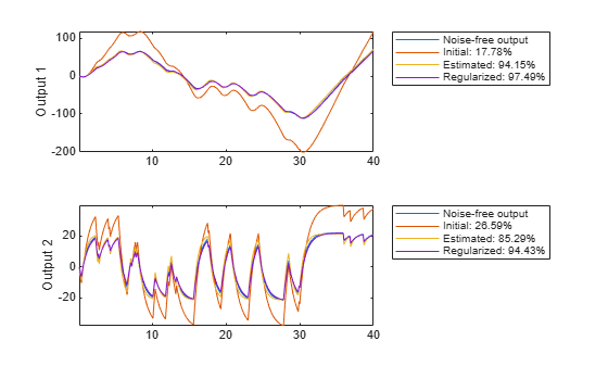
Figure contains 2 axes objects. Axes object 1 with ylabel Output 1 contains 4 objects of type line. These objects represent Noise-free output, Initial: 17.78%, Estimated: 94.15%, Regularized: 97.49%. Axes object 2 with ylabel Output 2 contains 4 objects of type line. These objects represent Noise-free output, Initial: 26.59%, Estimated: 85.29%, Regularized: 94.43%.

図 18: ノイズのない測定出力と、初期モデル、推定モデル、正則化モデルのモデル出力

正則化した推定では、正則化していない推定と比較してパラメーターの分散が小さくなっています。これは、mr のボード線図の信頼限界が、m のボード線図の信頼限界よりも狭いことで示されます。

clf
showConfidence(bodeplot(m,mr,logspace(-1,1.4,100)),3) % 3 s.d. region
legend('show')

MATLAB figure

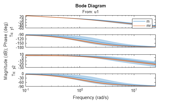
図 19: 信頼限界付きの m と mr のボード線図

これは、事前情報と測定情報の結合がどのように機能するかを示したものです。実際には、既存の情報源に合わせて Lambda のサイズを調整する手順が必要です。一般的に使用される方法では、"交差検定" を使用します。つまり、以下のようにします。

データを推定データと検証データの 2 つの部分に分ける。
推定データを使用して、さまざまな Lambda の値について正則化モデルを計算する。
モデルがどれぐらい検証データをよく再現しているかを評価する。compare コマンドまたは goodnessOfFit コマンドで得られた NRMSE 適合値を表にする。
モデルが検証データに最もよく適合する Lambda を選択する。

大規模な非線形モデルをロバストにするための正則化の使用

正則化のもう 1 つの用途は、大規模 (多くの場合非線形) モデルの推定を数値的に安定にすることです。非線形ダイナミクスをもつデータレコード nldata を用意しました。多数のユニットをもつニューラルネットワーク特性の非線形 ARX モデルを試します。

load regularizationExampleData.mat nldata
opt = nlarxOptions('SearchMethod','lm');
m10 = nlarx(nldata, [1 2 1], idSigmoidNetwork(10), opt);
m20 = nlarx(nldata, [1 2 1], idSigmoidNetwork(20), opt);
m30 = nlarx(nldata, [1 2 1], idSigmoidNetwork(30), opt);

compare(nldata, m10, m20) % compare responses of m10, m20 to measured response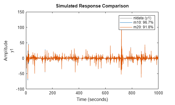

MATLAB figure

図 20: m10 と m20 のモデルの比較プロット

fprintf('Number of parameters (m10, m20, m30): %s\n',...
   mat2str([nparams(m10),nparams(m20),nparams(m30)]))

Number of parameters (m10, m20, m30): [54 104 154]

compare(nldata, m30, m10, m20) % compare all three models
axis([1 800 -57 45])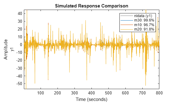

MATLAB figure

図 21: m10、m20、m30 のモデルの比較プロット

最初の 2 つのモデルは、良好で改善された適合を示します。しかし、m30 の 154 個のパラメーターを推定すると、数値的な問題が発生しているように見えます。このため、正則化を少し適用することで、より優れた条件付き行列を得ることができます。

opt.Regularization.Lambda = 1e-8;
m30r = nlarx(nldata, [1 2 1], idSigmoidNetwork(30), opt);
compare(nldata, m30r, m10, m20)

MATLAB figure

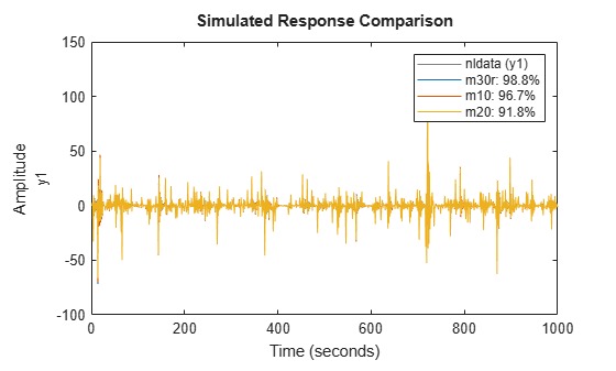
図 22: m10、m20 のモデルと m30r の正則化モデルの比較プロット

ニューロンを 30 個もつモデルで、推定データの適合が大幅に改善されました。前述したように、使用する Lambda 値を系統的に検索するには交差検定テストが必要です。

まとめ

FIR モデル、線形グレーボックスモデル、非線形 ARX モデルの推定における正則化の利点について説明しました。正則化定数の Lambda と R を適切に選択した場合、正則化により同定モデルの品質に大きな影響を与えることができます。ARX モデルの場合、これは関数 arxRegul を使用することでとても簡単に行えます。また、これらの自動選択の値が、専用の状態空間推定アルゴリズム ssregest に入力されます。

その他の種類の推定の場合、Lambda を決定するには交差検定ベースの検索を行わなければなりません。グレーボックスモデルのような構造化されたモデルの場合、R を使用して、対応するパラメーターの初期値の信頼性を指定することができます。次に、正則化の Nominal オプションを使用して、パラメーター値の事前情報とデータの情報をマージすることができます。

正則化オプションは、伝達関数とプロセスモデル、状態空間モデルと多項式モデル、非線形 ARX、Hammerstein-Wiener と線形/非線形のグレーボックスモデルなど、すべての線形モデルおよび非線形モデルで使用できます。

動的システムの正則化による同定

正則化とは

FIR モデリングでのバイアスと分散のトレードオフ

FIR モデルの正則化定数の自動決定

正則化 ARX モデルによる状態空間モデルの推定

低次元化による正則化手法を使用した状態空間モデルの推定

グレー ボックス モデルの基本的なバイアスと分散のトレードオフ

大規模な非線形モデルをロバストにするための正則化の使用

まとめ

グレーボックスモデルの基本的なバイアスと分散のトレードオフ