Picking Instrumental Variables for System Identification
This example provides a simple illustration of the meaning and choice of instrumental variables (IVs) for system identification. In the System Identification Toolbox™, the ARX model estimation using the least-squares approach is performed using the arx command, while the instrumental variable based technique is used in the following functions:
ivx- where you can provide arbitrary signal x(t) for the instrumentsiv4- same as ivx but the optimal instruments are determined automaticallyivar- AR/ARMA model for time-series data; instruments are chosen automatically
Introduction
An identification problem typically involves determining the coefficients of a difference- or differential-equation that relates certain measured input u(t) to the measured output y(t). Such an equation is commonly denoted by a model such as a transfer function, a polynomial model, or a state-space model. An example is the ARX model:
where are polynomial composed of linear delay operators, and are unmeasured disturbances typically described as a Gaussian white noise of zero mean and a constant variance (an i.i.d. sequence). If we pick , the resulting ARX model is:
, or:
... (1)
Another example is an Output-Error (OE) model, typically, referred to as a discrete-time transfer function:
For , the difference equation corresponding to this structure is:
... (2)
About Instrumental Variables
A simple, but practical view of the instrumental variables is that they are auxiliary signals (as such different from or ). That helps compensate for the effect of disturbances in determining accurate estimates of the model parameters (i.e., the constants in the ARX and OE models above). The motivation behind the choice of is to correlate out the effect of disturbance from the equations. This is best seen when using the correlation based approach to solving stochastic difference equations. For example, multiply both the side of equation (1) with random variable and compute expectations. This gives:
where is the expectation operator. The expectation can be computed as a sample mean of the quantities over a given time range. For example, if the measurements of are available over a time range of seconds, then:
where denotes the correlation between the variables and . The correlation equation then takes the form:
... (3)
Suppose we pick to be , that is, the output variables shifted by one sample. Then we get:
Since we can typically assume that is uncorrelated with , we have . Thus we have managed to correlate out the effect of in equation (3) by pick the instrumental variable as . Of course, this is not the only possible choice for . It can be any signal that shows strong correlation with the output but is uncorrelated with the disturbance .
Identification of ARX Models
Given samples of input and output signals over a time range, we need to solve for the coefficients of the delay operator polynomials . In ARX equation (1) we can minimize the sum of squared errors over a time span, that is, minimize . Since equation (1) is linear in the unknowns, minimization of can be achieved using linear least squares, typically performed using the backslash ("\") operator in MATLAB®. Define the regressor matrix as a matrix composed of the observations of , and the vector of output observations, that is:
then we have:
,
where is the vector of unknowns. Given numeric values for matrices , we can solve for as . In most cases, the backslash operator computes the least squares solution . This is the solution approach used by the arx command.
Stochastic Difference Equation Based Approach to Estimation
Note that the least-squares solution can be written as:
where is the vector of model regressors. The two summations can be viewed as correlation matrices:
This means that the least-squares solution can also be derived by using the correlation approach, where we pick , and as instrumental variables. In particular, using as the first instrumental variable the correlation equation (obtained by multiplying both sides of the equation (1) by and taking expectation) becomes:
.... 4(a)
Using as the instrumental variable gives:
.... 4(b)
Equations 4(a), and 4(b) can be solved simultaneously to obtain the estimates of the unknowns and Thus the standard ARX algorithm amounts to picking the regressors themselves as the instrumental variables.
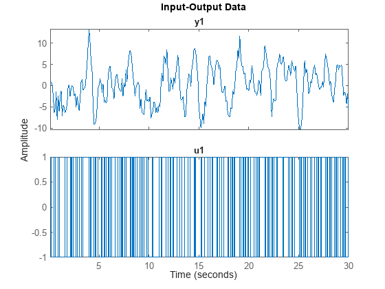
% Load input/output data from a SISO system
load IODataForIVExample IOData
idplot(IOData)
% Estimate an ARX Model of order na = 2, nb = 2, nk = 1. This amounts to using the regressors
% y(t-1), y(t-2), u(t-1), u(t-2)
na = 2;
nb = 2;
nk = 1;
sysARX = arx(IOData,[na nb nk])
sysARX =
Discrete-time ARX model: A(z)y(t) = B(z)u(t) + e(t)
  A(z) = 1 - 0.8281 z^-1 + 0.09117 z^-2

  B(z) = 0.8454 z^-1 + 1.233 z^-2

Sample time: 0.1 seconds

Parameterization:
   Polynomial orders:   na=2   nb=2   nk=1
   Number of free coefficients: 4
   Use "polydata", "getpvec", "getcov" for parameters and their uncertainties.

Status:
Estimated using ARX on time domain data "IOData".
Fit to estimation data: 53.67% (prediction focus)
FPE: 4.55, MSE: 4.371

Model Properties
Now estimate a model using the instrumental variable approach. Use the model regressors as the 4 instrumental variables. For the ARX model, the IV solution takes the form:
where is the vector of instrumental variables. For the ivx command, the instrumental variable information is provided using the third input argument X.
You do not need to generate the regressor data manually. You can simply provide a filtered version of the output signals to be used for generating the instrumental variables. The ivx command automatically generates the output related instruments by shifting the provided signal according to the na value. For example, if na=2, then the ivx command internally generates X(t-1), X(t-2) as instrumental variables. For this example, X is same as the measured output - IOData.y1.
Note also that the shifted versions of the input signal are automatically added in accordance to the value of nb and nk. Thus if nb=2, nk=1, then the ivx command internally generates u(t-1), u(t-2) and adds them to the list of instrumental variables.
X = IOData.y1;
% X is the signal from which the first 2 IVs are generated.
% The other 2 are automatically added using the input signal IOData.u1.
sysIV = ivx(IOData, [na nb nk], X)
sysIV =
Discrete-time ARX model: A(z)y(t) = B(z)u(t) + e(t)
  A(z) = 1 - 0.8281 z^-1 + 0.09117 z^-2

  B(z) = 0.8454 z^-1 + 1.233 z^-2

Sample time: 0.1 seconds

Parameterization:
   Polynomial orders:   na=2   nb=2   nk=1
   Number of free coefficients: 4
   Use "polydata", "getpvec", "getcov" for parameters and their uncertainties.

Status:
Estimated using IVX on time domain data "IOData".
Fit to estimation data: 53.67% (prediction focus)
FPE: 4.55, MSE: 4.371

Model Properties
As seen by this exercise, sysIV matches sysARX. Thus using the output signal itself as the instrumental variable generator, we can reproduce the least-squares solution of the arx command. We can verify these results by manual computation. Note that is the vector of unknowns.
%The GETREG command can be used for quickly generating the regressor data.
vars = IOData.Properties.VariableNames;
L = linearRegressor(vars,1:2);
D = getreg(L,IOData);
head(D)
Time u1(t-1) u1(t-2) y1(t-1) y1(t-2)
_______ _______ _______ _______ _______
0.1 sec NaN NaN NaN NaN
0.2 sec 1 NaN 0.39221 NaN
0.3 sec -1 1 0.84255 0.39221
0.4 sec -1 -1 0.3107 0.84255
0.5 sec -1 -1 -2.3174 0.3107
0.6 sec 1 -1 -6.3138 -2.3174
0.7 sec -1 1 -5.4381 -6.3138
0.8 sec -1 -1 -1.5059 -5.4381
% The NaNs in the first two rows of D correspond to the unknown initial conditions. Remove them.
D = D(3:end,:);

% For linear regression, the corresponding response values are:
Y = IOData.y1(3:end);

% The ARX command computes the parameters by least squares.
Theta = D{:,:}\Y;
a = [1, -Theta(3:4)']; % the A(q) polynomial
b = [0, Theta(1:2)'];  % the B(q) polynomial
%
disp('A(q) values')
A(q) values
disp([a; sysARX.a])
    1.0000   -0.8281    0.0912
    1.0000   -0.8281    0.0912
%
disp('B(q) values')
B(q) values
disp([b; sysARX.b])
         0    0.8454    1.2331
         0    0.8454    1.2331
The value of a matches sysARX.a. Similarly, the values of b and sysARX.b match. The Examples section below explores other choices of instruments.
Example: Exploring Choice of Optimal Instruments for ARX Models
Using redundant sensor measurement as instrumental variable
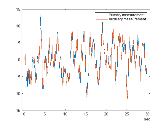
Suppose the experimental setup allows multiple measurements of the output signal. For example, an audio signal can be measured by sensors at two nearby locations. This way, both sensors measure the same signal but are corrupted by noise independently of each other. The variable y2 represents the output value measured using an auxiliary sensor.
load IODataForIVExample y2
t = IOData.Properties.RowTimes;
plot(t,IOData.y1, t,y2)
legend('Primary measurement', 'Auxiliary measurement')
Use y2 as instrumental variable generating signal.
sysIV2 = ivx(IOData, [na nb nk], y2)
sysIV2 =
Discrete-time ARX model: A(z)y(t) = B(z)u(t) + e(t)
  A(z) = 1 - 1.169 z^-1 + 0.4005 z^-2

  B(z) = 0.8912 z^-1 + 0.9849 z^-2

Sample time: 0.1 seconds

Parameterization:
   Polynomial orders:   na=2   nb=2   nk=1
   Number of free coefficients: 4
   Use "polydata", "getpvec", "getcov" for parameters and their uncertainties.

Status:
Estimated using IVX on time domain data "IOData".
Fit to estimation data: 50.05% (prediction focus)
FPE: 5.287, MSE: 5.08

Model Properties
Using instruments automatically generated by IV4
The iv4 command automatically determines optimal instruments to use based on certain assumptions regarding the nature of the system and the disturbances. You can call iv4 with the same input arguments as used for the arx command.
% Identify a model of the same order as before using the IV4 command
sysOpt = iv4(IOData, [na nb nk])
sysOpt =
Discrete-time ARX model: A(z)y(t) = B(z)u(t) + e(t)
A(z) = 1 - 1.506 z^-1 + 0.7088 z^-2
B(z) = 0.9258 z^-1 + 0.6223 z^-2
Sample time: 0.1 seconds
Parameterization:
Polynomial orders: na=2 nb=2 nk=1
Number of free coefficients: 4
Use "polydata", "getpvec", "getcov" for parameters and their uncertainties.
Status:
Estimated using IV4 on time domain data "IOData".
Fit to estimation data: 40.55% (prediction focus)
FPE: 7.491, MSE: 7.197
Model Properties
sysOpt has worse 1-step prediction accuracy than sysARX, or sysIV. However it performs better on long-horizon predictions. Similarly, sysIV2 performs better for longer-term predictions.
% compare model performance for long-term (infinity horizon) predictions
compare(IOData, sysARX, sysIV, sysIV2, sysOpt)
The results can be validate further on an independent dataset as described in the Model Validation section.
Identification of Output-Error (OE) Models
The ARX estimation technique provides correct estimates of the model parameters if the disturbances are indeed equation errors, that is, they match the manner in which affects the output . However, in many situations, this is not the case. The simplest example is where the unmeasured disturbances are owing to sensor measurement noise. In this case, the true system takes the form:
that is, the output-error form. In this case, the arx command leads to biased estimates of the model parameters. The correct estimator to use in this case is the oe function. Here is an example:
sysOE = oe(IOData, [nb na nk])
sysOE =
Discrete-time OE model: y(t) = [B(z)/F(z)]u(t) + e(t)
  B(z) = 0.9447 z^-1 + 0.5256 z^-2

  F(z) = 1 - 1.539 z^-1 + 0.7313 z^-2

Sample time: 0.1 seconds

Parameterization:
   Polynomial orders:   nb=2   nf=2   nk=1
   Number of free coefficients: 4
   Use "polydata", "getpvec", "getcov" for parameters and their uncertainties.

Status:
Estimated using OE on time domain data "IOData".
Fit to estimation data: 63.5%
FPE: 2.786, MSE: 2.712

Model Properties
The oe command estimates the coefficients of the numerator and the denominator polynomials by minimizing the sum of squares of the errors , . However, the minimization objective is non-convex in the model parameters. The minimization uses iterative numerical minimization techniques. This is significantly more complicated than the simple least-squares approach used by the arx algorithm. Moreover, best results are typically not guaranteed since the minimization algorithms can get stuck at a local minima of . The results obtained by oe can be different depending upon the choice of the initial values of the parameters, the choice of the search method and its configuration.
Can a suitable choice of instrumental variables avoid the estimation bias and deliver the correct results while still using the non-iterative computation method of IV algorithms? Note that the OE model can be written as:
which has ARMAX structure with . For na=nb=2, nk=1, this model takes the form:
To correlate out the influence of errors at a give time , we can use a IV variable with a lag of at least 3. Another option is to use a variable that is not completely uncorrelated with the errors but then accounting for the effect of the correlations explicitly. These choices are explored next.
Using Instruments with Lags Larger than the Model Order
For the current example, the model order is . A candidate IV set is: . This can be achieved by using in the ivx command.
sysIV_OE = ivx(IOData(3:end,:), [na nb nk], IOData.y1(1:end-2))
sysIV_OE =
Discrete-time ARX model: A(z)y(t) = B(z)u(t) + e(t)
  A(z) = 1 - 1.577 z^-1 + 0.7681 z^-2

  B(z) = 0.9414 z^-1 + 0.6868 z^-2

Sample time: 0.1 seconds

Parameterization:
   Polynomial orders:   na=2   nb=2   nk=1
   Number of free coefficients: 4
   Use "polydata", "getpvec", "getcov" for parameters and their uncertainties.

Status:
Estimated using IVX on time domain data.
Fit to estimation data: 38.18% (prediction focus)
FPE: 8.157, MSE: 7.835

Model Properties
We can verify this result by manual computations using the correlations matrices.
% generate regressors data for [y(t-1), ..., y(t-4), u(t-1), u(t-2)]
L = linearRegressor(vars,{1:2,1:4});
D = getreg(L,IOData);
head(D)
Time u1(t-1) u1(t-2) y1(t-1) y1(t-2) y1(t-3) y1(t-4)
_______ _______ _______ _______ _______ _______ _______
0.1 sec NaN NaN NaN NaN NaN NaN
0.2 sec 1 NaN 0.39221 NaN NaN NaN
0.3 sec -1 1 0.84255 0.39221 NaN NaN
0.4 sec -1 -1 0.3107 0.84255 0.39221 NaN
0.5 sec -1 -1 -2.3174 0.3107 0.84255 0.39221
0.6 sec 1 -1 -6.3138 -2.3174 0.3107 0.84255
0.7 sec -1 1 -5.4381 -6.3138 -2.3174 0.3107
0.8 sec -1 -1 -1.5059 -5.4381 -6.3138 -2.3174
% remove first 4 rows that contain the effect of initial conditions
D = D(5:end,:);
Phi = D{:,1:4}; % u(t-1), u(t-2), y(t-1), y(t-2)
IV = D{:,[1 2 5 6]}; % u(t-1), u(t-2), y(t-3), y(t-4)
Y = IOData.y1(5:end);
Theta = (IV'*Phi)\(IV'*Y)
Theta = 4×1

     0.9414
     0.6868
     1.5766
    -0.7681
a = [1, -Theta(3:4)'] % A(q), matches sysIV_OE.aa = 1×3
1.0000 -1.5766 0.7681
b = [0, Theta(1:2)'] % B(q), matches sysIV_OE.bb = 1×3
0 0.9414 0.6868
% check model performance for inf-horizon prediction
compare(IOData, sysARX, sysOE, sysIV_OE, sysOpt)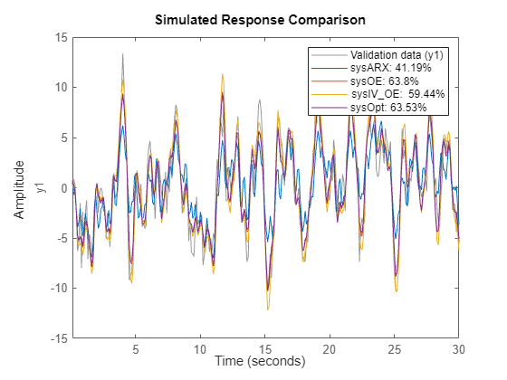
sysIV_OE does better than sysARX but still not as good as sysOE. However, sysOpt, which was estimated with automatically chosen instruments, matches the performance of sysOE.
Using Error-Correlated Instrumental Variables
Under the assumption that , for , is an identically distributed sequence of independent random variables: , where is typically unknown.
.
Using the IVs that are the same as the model regressors, we get the following correlation equations:
The presence of the unknown in the first two equations means that a linear least-squares solution cannot be used (there are terms involving products of unknowns). This removes the benefit of using instrumental variables; ivx cannot overcome the effect of this correlation if using .
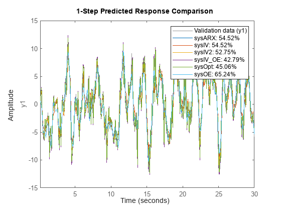
Model Validation
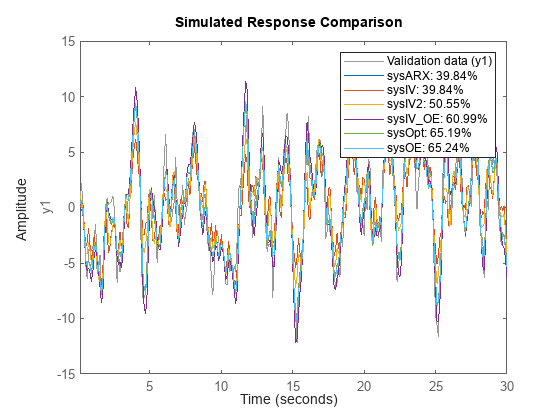
% Create a validation dataset using the output signal from the auxiliary sensor.
vData = IOData;
vData.y1 = y2;
% compare 1-step ahead prediction performance
compare(vData, sysARX, sysIV, sysIV2, sysIV_OE, sysOpt, sysOE, 1)
% compare 10-step ahead prediction performance
compare(vData, sysARX, sysIV, sysIV2, sysIV_OE, sysOpt, sysOE, 10)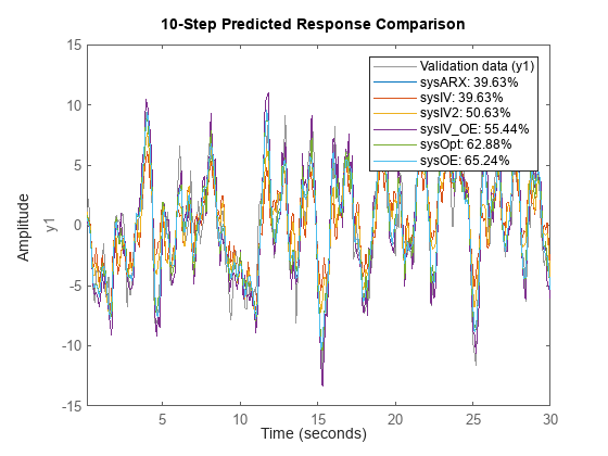
% compare infinite-horizon performance of the models
compare(vData, sysARX, sysIV, sysIV2, sysIV_OE, sysOpt, sysOE)