ガラス管製造工程

実験データ

まず、iddata オブジェクトとして保存されている入力データと出力データを読み込むことから始めます。

load thispe25.mat

データは変数 glass に格納されています。

glass

glass =

Time domain data set with 2700 samples.
Sample time: 1 seconds                  
                                        
Outputs      Unit (if specified)        
   Thickn                               
                                        
Inputs       Unit (if specified)        
   Speed                                
                                        

データには、1 つの入力 (Speed) と 1 つの出力 (Thickn) のサンプルが 2700 個含まれています。サンプル時間は 1 秒です。

このデータを推定用と交差検定用の 2 つに分割します。

ze = glass(1001:1500); %Estimation data
zv = glass(1501:2000,:); %Validation data

推定データのクローズアップ表示:

plot(ze(101:200)) %Plot the estimation data range from samples 101 to 200.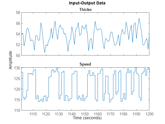

データの予備解析

最初の前処理ステップとして平均値を削除します。

ze = detrend(ze);
zv = detrend(zv);

データのサンプル時間は 1 秒ですが、工程の時定数はそれよりはるかに遅い可能性があります。出力では、むしろ高い周波数が検出される可能性があります。これを確認するために、最初に入力と出力のスペクトルを計算します。

sy = spa(ze(:,1,[]));
su = spa(ze(:,[],1));
clf
spectrum(sy,su)
axis([0.024 10 -5 20])
legend({'Output','Input'})
grid on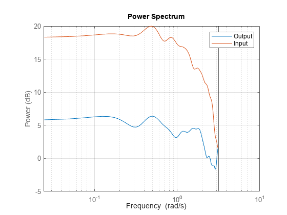

入力は 1 ラジアン/秒以上で非常に小さい相対エネルギーをもつのに対し、出力はその周波数以上で相対的に大きな値を含むことに注目してください。したがって、モデル作成にとって問題を引き起こす可能性がある高周波数外乱があります。

入力から出力までの潜在的フィードバックおよび遅延について洞察を得るために、データの一部を使用してインパルス応答を計算します。

Imp = impulseest(ze,[],'negative',impulseestOptions('RegularizationKernel','SE'));
showConfidence(impulseplot(Imp,-10:30),3)
grid on

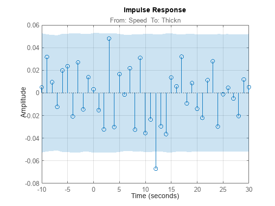
インパルス応答に約 12 サンプルの遅延が見られます (信頼区間外での最初の重要な応答値)。また、負の時間ラグにとってもインパルス応答は重要です。これはデータ内にフィードバックがある確率が高いことを示し、出力の将来値が現在の入力に影響する (追加される) ことを意味します。入力遅延は delayest を使って明示的に計算できます。

delayest(ze)

ans = 12

フィードバックの確率は feedback を使って求めることができます。

feedback(ze) %compute probability of feedback in data

ans = 100

したがって、データ内にフィードバックが存在することはほぼ確実です。

さらに、予備テストとしてスペクトル解析推定値を計算します。

g = spa(ze);
showConfidence(bodeplot(g))
grid on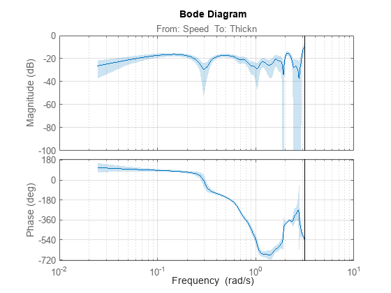

特に、高周波数での動作は非常に不確実です。モデルの範囲を 1 ラジアン/秒より低く抑えるのが賢明でしょう。

工程の動作のパラメトリック モデル

推定データを使って 4 次の ARX モデルを計算し、検証データを使ってそのモデルをシミュレートすることで、適切なダイナミクスを導き出せるかどうか簡単にチェックしてみましょう。遅延が約 12 秒であることがわかっています。

m1 = arx(ze,[4 4 12]);
compare(zv,m1);

シミュレーション結果の詳細:

compare(zv,m1,inf,'Samples',101:200)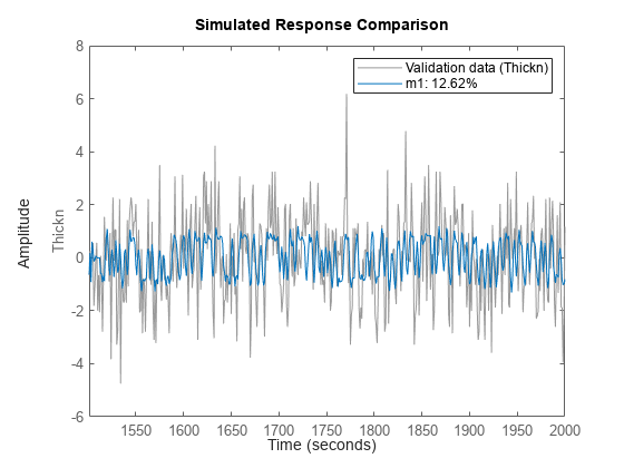

出力の高周波数成分の処理には明らかに問題があります。その問題に加えて、長い遅延もあるため、データを 4 で間引く (つまり、ローパス フィルターを使って値を 4 つごとに 1 つ拾い上げる) のが得策です。

if exist('resample','file')==2
    % Use "resample" command for decimation if Signal Processing Toolbox(TM)
    % is available.
    zd = resample(detrend(glass),1,4,20);
else
    % Otherwise, use the slower alternative - "idresamp"
    zd  = idresamp(detrend(glass),4);
end
   
zde = zd(1:500);
zdv = zd(501:size(zd,'N'));

間引かれたデータに適した構造を見つけましょう。最初にインパルス応答を計算します。

Imp = impulseest(zde);
showConfidence(impulseplot(Imp,200),3)
axis([0  100  -0.05  0.01])
grid on

ここでも、約 3 サンプルの遅延が見られます (zde においてサンプル時間 4 秒に対して 12 秒の遅延なので、これは前述の現象と一貫しています)。今度は既定のモデルを推定してみましょう。次数は推定器によって自動的に選択されます。

Mdefault = n4sid(zde);
compare(zdv,Mdefault)

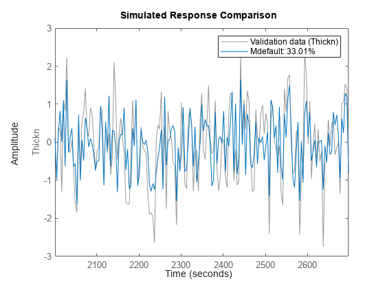
推定器は 4 次モデルを選択しました。これは間引きされていないデータ用のモデルより適切なモデルであるように見えます。ここで、どのようなモデル構造と次数を使用できるかを体系的に評価しましょう。最初に遅延を調べます。

V = arxstruc(zde,zdv,struc(2,2,1:30));
nn = selstruc(V,0)

nn = 1×3

     2     2     3

ARXSTRUC は、インパルス応答からの測定値と一致する 3 サンプルの遅延も提示しています。したがって、遅延を 3 の近傍に固定し、この遅延の周りでいくつかの異なる次数をテストすることにします。

V = arxstruc(zde,zdv,struc(1:5,1:5,nn(3)-1:nn(3)+1));

ここで、最も好ましいモデル次数 (V の最初の行に表示される最小損失関数) を選択するために、返された行列に対して selstruc を呼び出します。

nn = selstruc(V,0); %choose the "best" model order

SELSTRUC は、次数選択の対型モードを起動するために入力を 1 つだけ指定して呼び出すこともできます (nn = selstruc(V))。

変数 nn で返された "最良" の次数を使ったモデルを計算してチェックしてみましょう。

m2 = arx(zde,nn);
compare(zdv,m2,inf,compareOptions('Samples',21:150));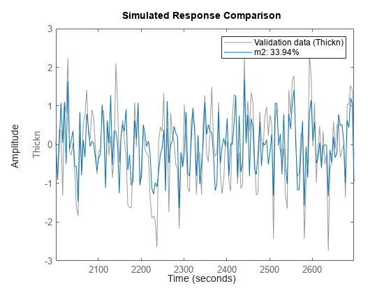

モデル m2 は Mdefault とほぼ同じで、データを適合しますが低い次数を使用します。

残差をテストしてみましょう。

resid(zdv,m2);

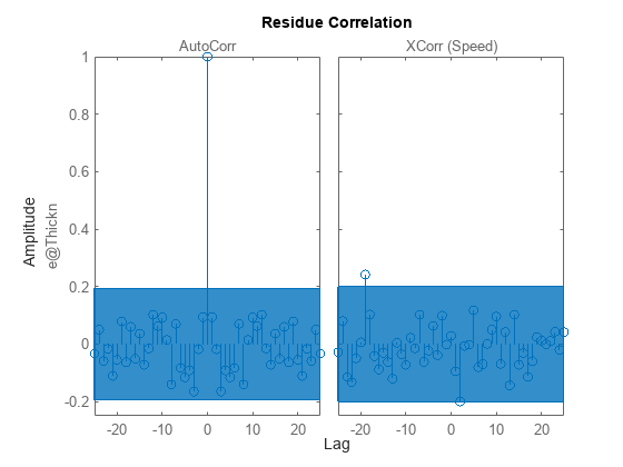
残差は信頼区間領域内にあり、主要なダイナミクスがモデルによって再現されたことを示しています。この極-零点図は何を意味しているのでしょうか。

clf
showConfidence(iopzplot(m2),3)
axis([ -1.1898,1.3778,-1.5112,1.5688])

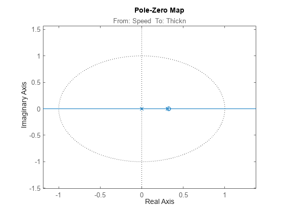
極-零点プロットは、複数のペアで極-零点相殺が生じていることを示しています。これは、それらの位置が信頼領域内で重なっているためです。これは、次数が低いモデルの方が適していることを示しています。次の [1 1 3] ARX モデルを試してください。

m3 = arx(zde,[1 1 3])

m3 =
Discrete-time ARX model: A(z)y(t) = B(z)u(t) + e(t)
  A(z) = 1 - 0.115 z^-1                            
                                                   
  B(z) = -0.1788 z^-3                              
                                                   
Sample time: 4 seconds
  
Parameterization:
   Polynomial orders:   na=1   nb=1   nk=3
   Number of free coefficients: 2
   Use "polydata", "getpvec", "getcov" for parameters and their uncertainties.

Status:                                          
Estimated using ARX on time domain data "zde".   
Fit to estimation data: 35.07% (prediction focus)
FPE: 0.4437, MSE: 0.4384                         
 

モデル m3 のシミュレーションを検証データと比較した結果は次のとおりです。

compare(zdv,Mdefault,m2,m3)

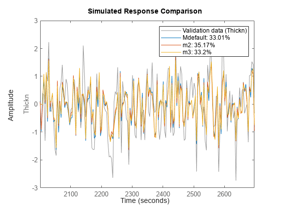
これら 3 つのモデルは比較可能な結果を提示しています。同様に、これらモデルの 5 ステップ先を予測する機能を比較できます。

compare(zdv,Mdefault,m2,m3,5)

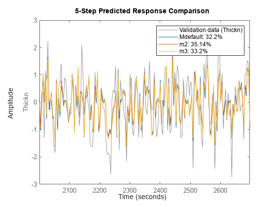
これらのプロットが示すように、モデル次数の低次元化は、将来値を予測するモデルの有効性を大きく低下させることはありません。