タイミングオフセットの推定

この例では、MATLAB® コードで実装された基本的なリードラグタイミングオフセット推定アルゴリズムからの HDL コードの生成方法を示します。

はじめに

無線通信システムの RF フロントエンドで受信データがオーバーサンプリングされています。これは、受信フィルターのために十分なサンプリングレートを提供するなど、いくつかの目的を果たします。

その中でも最も重要な役割の 1 つは、受信波形の最大振幅点の近くでデータをサンプリングできるように、受信波形で複数のサンプリング点を提供することです。この例では、再帰的に動作する基本的なリードラグ時間オフセット推定コアを示します。

この設計で生成されるハードウェアコアは 1/os_rate で動作します。os_rate はオーバーサンプリングレートです。つまり、このコアはオーバーサンプリングされた 8 クロックサイクルごとに 1 回反復されます。出力はシンボルレートです。

design_name = 'mlhdlc_comms_toe';
testbench_name = 'mlhdlc_comms_toe_tb';

この MATLAB® 設計を見てみましょう。

type(design_name);

%%%%%%%%%%%%%%%%%%%%%%%%%%%%%%%%%%%%%%%%%%%%%%%%%%%%%%%%%%%%%%%%%%%%%%%%%%%
% MATLAB design: Time Offset Estimation
%
%% Introduction:
%
% The generated hardware core for this design operates at 1/os_rate 
% where os_rate is the oversampled rate. That is, for 8 oversampled clock cycles 
% this core iterates once. The output is at the symbol rate.
%
% Key design pattern covered in this example:
% (1) Data is sent in a vector format, stored in a register and accessed
% multiple times
% (2) The core also illustrates basic mathematical operations
% 

%   Copyright 2011-2015 The MathWorks, Inc.

%#codegen
function [tauh,q] = mlhdlc_comms_toe(r,mu)

persistent tau
persistent rBuf

os_rate = 8;
if isempty(tau)
    tau = 0;
    rBuf = zeros(1,3*os_rate);
end

rBuf = [rBuf(1+os_rate:end) r];

taur = round(tau);

% Determine lead/lag values and compute offset error
zl = rBuf(os_rate+taur-1);
zo = rBuf(os_rate+taur);
ze = rBuf(os_rate+taur+1);
offsetError = zo*(ze-zl);

% update tau
tau = tau + mu*offsetError;

tauh = tau;

q = zo;

type(testbench_name);

function mlhdlc_comms_toe_tb
%

%   Copyright 2011-2015 The MathWorks, Inc.

os_rate = 8;
Ns = 128;
SNR = 100;
mu = .5; % smoothing factor for time offset estimates

% create simulated signal
rng('default'); % always default to known state  
b = round(rand(1,Ns));
d = reshape(repmat(b*2-1,os_rate,1),1,Ns*os_rate);

x = [zeros(1,Ns*os_rate) d zeros(1,Ns*os_rate)];
y = awgn(x,SNR);

w = fir1(3*os_rate+1,1/os_rate)';
z = filter(w,1,y);
r = z(4:end); % give it an offset to make things interesting

%tau = 0;
Nsym = floor(length(r)/os_rate);
tauh = zeros(1,Nsym-1); q = zeros(1,Nsym-1);
for i1 = 1:Nsym-1
    rVec = r(1+(i1-1)*os_rate:i1*os_rate);
    
    % Call to the Timing Offset Estimation Algorithm
    [tauh(i1),q(i1)] = mlhdlc_comms_toe(rVec,mu);
end

indexes = 1:os_rate:length(tauh)*os_rate;
indexes = indexes+tauh+os_rate-1-os_rate*2;

Fig1Loc=figposition([5 50 90 40]);
H_f1=figure(1); clf;
set(H_f1,'position',Fig1Loc);
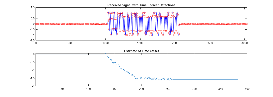
subplot(2,1,1)
plot(r,'b');
hold on
plot(indexes,q,'ro');
axis([indexes(1) indexes(end) -1.5 1.5]);
title('Received Signal with Time Correct Detections');
subplot(2,1,2)
plot(tauh);
title('Estimate of Time Offset');

function y=figposition(x)
%FIGPOSITION Positions figure window irrespective of the screen resolution
% Y=FIGPOSITION(X) generates a vector the size of X. 
% This specifies the location of the figure window in pixels
% 
screenRes=get(0,'ScreenSize');
% Convert x to pixels
y(1,1)=(x(1,1)*screenRes(1,3))/100;
y(1,2)=(x(1,2)*screenRes(1,4))/100;
y(1,3)=(x(1,3)*screenRes(1,3))/100;
y(1,4)=(x(1,4)*screenRes(1,4))/100;

設計のシミュレーション

コードの生成前にテストベンチを使用して設計のシミュレーションを実行し、実行時エラーが発生しないことを常に確認することをお勧めします。

mlhdlc_comms_toe_tb

HDL Coder™ プロジェクトの新規作成

coder -hdlcoder -new mlhdlc_toe

次に、mlhdlc_comms_toe.m ファイルを MATLAB 関数としてプロジェクトに追加し、mlhdlc_comms_toe_tb.m を MATLAB テストベンチとして追加します。

MATLAB HDL Coder プロジェクトの作成と入力に関する詳細なチュートリアルについては、MATLAB から HDL へのワークフロー入門を参照してください。

固定小数点変換と HDL コード生成の実行

[ワークフローアドバイザー] ボタンからワークフローアドバイザーを起動し、[コード生成] のステップを右クリックして [選択したタスクまで実行] オプションを選択し、最初から HDL コード生成までのすべてのステップを実行します。

コード生成ログのウィンドウにあるハイパーリンクをクリックして、生成された HDL コードを確認します。

タイミング オフセットの推定

はじめに

設計のシミュレーション

HDL Coder™ プロジェクトの新規作成

固定小数点変換と HDL コード生成の実行

タイミングオフセットの推定