Analyze Track and Detection Association Using Analysis Info
This example shows how to use the analysis info output of the trackerGNN and trackerJPDA System objects to derive useful quantities about the assignments between tracks and detections.
Scenario and simulation
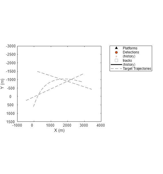
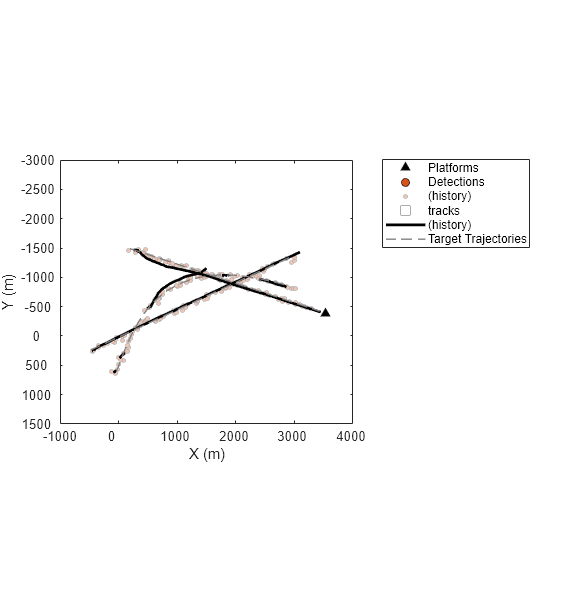
Create and simulate a simple tracking scenario and save the histories of detections, tracks, and analysis info. The scenario contains three targets with crossing trajectories. Targets are moving at a constant velocity. Use a monostatic radar sensor to generate positional detections of the targets.
scenario = createScenario();
[platp, detp, trackp] = createPlotters(scenario);
Create a trackerGNN object with the default configuration. Increase the association gate by setting the AssignmentThreshold property to 100 to preserve all possible associations.
tracker = trackerGNN(AssignmentThreshold=100);
detlog = {};
tracklog ={};
infolog = {};

rng(2022); %For repeatable results
while advance(scenario)
    % Generate sensor data
    [dets, configs, sensorConfigPIDs] = detect(scenario);

    % Update tracker
    [tracks, ~, ~, info] = tracker(dets, scenario.SimulationTime);

    % Update plots
    [truePosition, meas, meascov, trackpos, trackcov, trackids] = readData(scenario, dets, tracks);
    plotPlatform(platp,truePosition);
    plotDetection(detp,meas,meascov);
    plotTrack(trackp,trackpos,trackcov,trackids);
    drawnow

    % Log data
    detlog{end+1} = dets;
    tracklog{end+1} = tracks';
    infolog{end+1} = info; %#ok<*SAGROW>
end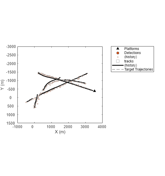
The figure above shows the detection and track history for the entire simulation. From the results, the tracker created multiple tracks but some targets were only partially tracked. To further understand the results, you can use the collected information to analyze the association between the detections and the tracks.
History of Assigned Detections for trackerGNN
You parse the info output to retrieve the list of detections associated to each track. First, you obtain the IDs of all the tracks.
alltrackids = unique(arrayfun(@(x) x.TrackID, [tracklog{:}]))alltrackids = 1×6 uint32 row vector
1 2 3 5 6 7
The tracker created six tracks during the simulation. Retrieve their assigned detections by querying the Assignment field of the info structure. Refer to the trackerGNN documentation for the definition of the Assignment matrix.
The function getDetectionHistoryGNN parses the info structure to find all the detections assigned to a given track. The function also returns the history of the tracks.
function [detHistory, trackHistory] = getDetectionHistoryGNN(infoLog, detLog, trackLog, tID)

detHistory = objectDetection.empty;
for i=1:numel(infoLog)

    curInfo = infoLog{i};
    existTrack = any(curInfo.TrackIDsAtStepBeginning == tID);
    if ~existTrack
        % Check if track was created
        if any(curInfo.InitiatedTrackIDs == tID)
            % Add initial detection
            detHistory(end+1) = detLog{i}{find(curInfo.InitiatedTrackIDs == tID)};
        end
        continue
    end

    if any(curInfo.DeletedTrackIDs == tID)
        %Track was deleted
        break
    end

    trackMatches = find(curInfo.Assignments(:,1) == tID );
    assignedDetectionIndices = curInfo.Assignments(trackMatches, 2);
    assignedDets = [detLog{i}{assignedDetectionIndices}];
    for j=1:numel(assignedDets)
        detHistory(end+1) =  assignedDets(j);
    end
end

trackarray = [trackLog{:}];
alltrackids = [trackarray.TrackID];
trackHistory = trackarray(alltrackids == tID);
Use this function and the plotTrackAndDets function, attached in the example folder, to find and display each track and its assigned detections in the same color.
tp = createHistoryPlotter();
for tid = alltrackids
    [detectionHistory, trackHistory] = getDetectionHistoryGNN(infolog,detlog,tracklog,tid);
    plotTrackAndDets(tp, detectionHistory, trackHistory);
end
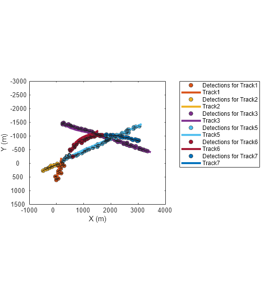
Zoom in on the region where the first track breaks. Observe that the yellow track (Track2) breaks because the detections along the true target trajectory are assigned to the orange track (Track1). Additionally, the yellow track fell behind the last two assigned detections, which can be attributed to poor velocity estimates. You can observe similar track breaks in the figure. Note that tuning the tracking filter can potentially improve the capability of the tracker on maintaining tracks through the trajectory crossing.
xlim([-543 654]);
ylim([-341 736]);
History of Assigned Detections for trackerJPDA
Simulate the same scenario but track targets using the trackerJPDA System object this time. Create the trackerJPDA object with the default tracking filter and the same assignment threshold as in the trackerGNN case.
tracker = trackerJPDA(AssignmentThreshold=100, ClutterDensity=5e-13, HitMissThreshold=0.1);

% Create a new plot
[platp, detp, trackp] = createPlotters(scenario);
hax = gca;

% Re-initialize logs
detlog = {};
tracklog ={};
infolog = {};

restart(scenario);
while advance(scenario)
    % Generate sensor data
    [dets, configs, sensorConfigPIDs] = detect(scenario);

    % Update tracker
    [tracks, ~, ~, info] = tracker(dets, scenario.SimulationTime);

    % Update plots
    [truePosition, meas, meascov, trackpos, trackcov, trackids] = readData(scenario, dets, tracks);
    plotPlatform(platp,truePosition);
    plotDetection(detp,meas,meascov);
    plotTrack(trackp,trackpos,trackcov,trackids);
    drawnow

    % Log data
    detlog{end+1} = dets;
    tracklog{end+1} = tracks';
    infolog{end+1} = info; %#ok<*SAGROW>
end
The figure above shows the tracking results. Similar to the results obtained with trackerGNN, the tracker creates multiple tracks and has a few track breaks. Next, you use the analysis info of trackerJPDA to analyze the association history.
The analysis info of trackerJPDA contains the clustering results. The helper function getDetectionHistoryJPDA shows one approach to parse the info and retrieve the list of detections used to correct each track. Unlike trackerGNN, trackerJPDA can assign multiple detections to multiple tracks, with different probabilistic weights. In this section, use the HitMissThreshold property of the tracker as the probability threshold to declare a detection assigned to a track.
function [detHistory, trackHistory] = getDetectionHistoryJPDA(infoLog, detLog, trackLog, tID, probThreshold)

detHistory = objectDetection.empty;
for i=1:numel(infoLog)

    curInfo = infoLog{i};
    existTrack = any(curInfo.TrackIDsAtStepBeginning == tID);
    isUnassigned = any(curInfo.UnassignedTracks == tID);
    if ~existTrack || isUnassigned
        % Check if track was created
        if any(curInfo.InitializedTrackIDs == tID)
            % Add initial detection
            detHistory(end+1) = detLog{i}{find(curInfo.InitializedTrackIDs == tID)};
        end
        continue
    end

    if any(curInfo.DeletedTrackIDs == tID)
        % Track was deleted
        break
    end

    % Find the cluster with tID
    hasTID = cellfun(@(x) any(x.TrackIDs == tID), curInfo.Clusters);
    cluster = curInfo.Clusters{hasTID};
    trackIndexInCluster = find(cluster.TrackIDs == tID );
    detIndexInCluster = find(cluster.MarginalProbabilities(1:end-1,trackIndexInCluster) > probThreshold);
    assignedDetectionIndices = cluster.DetectionIndices(detIndexInCluster);
    assignedDets = [detLog{i}{assignedDetectionIndices}];
    for j=1:numel(assignedDets)
        detHistory(end+1) =  assignedDets(j);
    end
end
trackLog = [trackLog{:}];
alltrackids = [trackLog.TrackID];
trackHistory = trackLog(alltrackids == tID);
In a new figure, visualize each track and its history of detections.
tp = createHistoryPlotter();
alltrackids = unique(arrayfun(@(x) x.TrackID, [tracklog{:}]));
for tid = alltrackids
    [detectionHistory, trackHistory] = getDetectionHistoryJPDA(infolog,detlog,tracklog,tid, tracker.HitMissThreshold);
    plotTrackAndDets(tp, detectionHistory, trackHistory);
end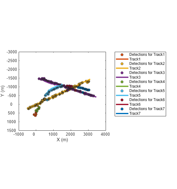
Assignment Cost and Assignment Probabilities
The cost matrix is another useful information in the info output of the tracker. In trackerJPDA, each cluster report contains the matrix of assignment probabilities. Use this information to visualize each cluster and quantify the contribution of each detection to each track update. The getClusterData function, attached in the example folder, shows how to parse the info output to obtain the number of clusters, a list of track reports for each cluster, a list of detections for each cluster, and their respective association probabilities.
function [numClusters, clusterTracks, clusterDetections, clusterProbabilities] = getClusterData(infolog, detlog, tracklog, step)

info = infolog{step};
detections = detlog{step};
numClusters = numel(info.Clusters);

% Retrieve tracks in cluster
initialTracks = tracklog{step -1};
clusterTracks = cell(1,numClusters);
clusterDetections = cell(1,numClusters);
clusterProbabilities = cell(1,numClusters);

for c=1:numClusters
    clusterTrackIDs = info.Clusters{c}.TrackIDs;
    clusterTracks{c} = initialTracks(ismember([initialTracks.TrackID],clusterTrackIDs));
    clusterDetections{c} = detections(info.Clusters{c}.DetectionIndices);
    clusterProbabilities{c} = info.Clusters{c}.MarginalProbabilities;
end
end
Next, use the getClusterData function to study the last track crossing which happens around step 59 of the simulation.
step = 59;
[numClusters, clusterTracks, clusterDetections, clusterProbabilities] = getClusterData(infolog, detlog, tracklog, step)
numClusters =
2
clusterTracks=1×2 cell array
    {1×2 objectTrack}    {1×1 objectTrack}
clusterDetections=1×2 cell array
    {1×2 objectDetection}    {1×1 objectDetection}
clusterProbabilities=1×2 cell array
    {3×2 double}    {2×1 double}
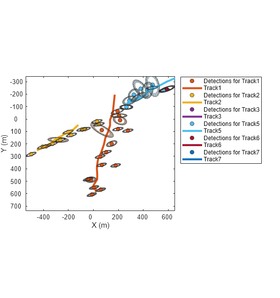
At this step, there were 2 clusters. The first cluster has 1 track and 1 detection. The second cluster has two tracks and two detections. Show the two clusters on a new figure.
f=figure(Units="normalized",OuterPosition=[0.2 0.2 0.45 0.6]);
newAx = copyobj(hax,f);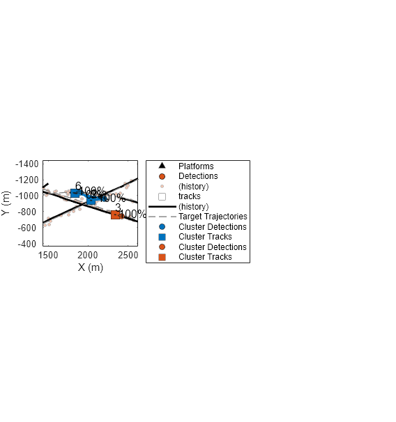
tp = theaterPlot("Parent",newAx);
xlim([1428 2625]);
ylim([-1442 -365]);
colors = lines(numClusters);
for c=1:numClusters
    plotCluster(tp, clusterTracks{c}, clusterDetections{c}, clusterProbabilities{c},colors(c,:));
end
Notice that Track 7 is only associated by 14% to one detection and 0 % to the second detection in its cluster. There is an 86% probability that the track was not associated to any detections.
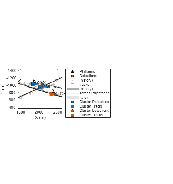
The animation below shows the evolution of the two clusters from step 50 to 60.
Conclusion
In this example you learned different ways to utilize the analysis info output of trackerGNN and trackerJPDA System objects to analyze the data association results. In particular, you learned how to retrieve the history of detections that constitutes a track and how to inspect joint track association clusters in the trackerJPDA System object.