アラン分散を使用した慣性センサーのノイズ解析
この例では、アラン分散を使用して MEMS ジャイロスコープのノイズ パラメーターを特定する方法を示します。これらのパラメーターは、ジャイロスコープをモデル化するためにシミュレーションで使用できます。ジャイロスコープの測定は次のようにモデル化されます。

3 つのノイズ パラメーター "N" (角度ランダム ウォーク)、"K" (レート ランダム ウォーク)、"B" (バイアス不安定性) は、静止状態のジャイロスコープから記録されたログ データを使用して推定されます。
背景
アラン分散は、David W. Allan によって、もともとは精密発振器の周波数安定性を測定するために開発されたものです。静止状態のジャイロスコープの測定に見られる各種ノイズ源の特定にも使用できます。サンプル時間  のジャイロスコープからのデータのサンプル数を "L" とします。期間 ,
  , ...,
  のデータ クラスターを形成し、各クラスターに含まれるデータ点の和をクラスターの長さで平均した値を取得します。アラン分散は、クラスター時間の関数としてのデータ クラスター平均の 2 標本分散と定義されます。この例では、オーバーラップするアラン分散推定器を使用します。これは、計算するクラスターがオーバーラップしていることを意味します。この推定器は、"L" の値が大きい場合に、オーバーラップのない推定器よりも優れた性能を示します。
アラン分散の計算
アラン分散は次のように計算されます。
サンプル周期 で "L" 個の静止状態のジャイロスコープ サンプルを記録します。 をログ サンプルとします。
% Load logged data from one axis of a three-axis gyroscope. This recording
% was done over a six hour period, with a 100 Hz sampling rate. The unit of
% the gyroscope data is in radians per second.
load('LoggedSingleAxisGyroscope', 'omega', 'Fs')
t0 = 1/Fs;
各サンプルについて、出力角度  を計算します。

離散サンプルについては、累積和に を乗算した値を使用できます。
theta = cumsum(omega, 1)*t0;
次に、アラン分散を計算します。
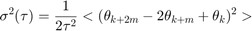
ここで、 と
と  はアンサンブル平均です。
アンサンブル平均は次のように展開できます。
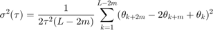
maxNumM = 100;
L = size(theta, 1);
maxM = 2.^floor(log2(L/2));
m = logspace(log10(1), log10(maxM), maxNumM).';
m = ceil(m); % m must be an integer.
m = unique(m); % Remove duplicates.

tau = m*t0;

avar = zeros(numel(m), 1);
for i = 1:numel(m)
    mi = m(i);
    avar(i,:) = sum( ...
        (theta(1+2*mi:L) - 2*theta(1+mi:L-mi) + theta(1:L-2*mi)).^2, 1);
end
avar = avar ./ (2*tau.^2 .* (L - 2*m));
最後に、アラン偏差  を使用してジャイロスコープのノイズ パラメーターを特定します。
adev = sqrt(avar);

figure
loglog(tau, adev)
title('Allan Deviation')
xlabel('\tau');
ylabel('\sigma(\tau)')
grid on
axis equal

アラン分散は allanvar 関数を使用して計算することもできます。
[avarFromFunc, tauFromFunc] = allanvar(omega, m, Fs);
adevFromFunc = sqrt(avarFromFunc);

figure
loglog(tau, adev, tauFromFunc, adevFromFunc);
title('Allan Deviations')
xlabel('\tau')
ylabel('\sigma(\tau)')
legend('Manual Calculation', 'allanvar Function')
grid on
axis equal

ノイズ パラメーターの特定
ジャイロスコープのノイズ パラメーターを取得するには、元のデータ セット におけるアラン分散とノイズ パラメーターの両側パワー スペクトル密度 (PSD) の関係を使用します。この関係は次のとおりです。
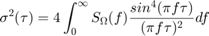
上記の方程式から、アラン分散は、伝達関数が  であるフィルターを通じて渡されるときのジャイロスコープの合計ノイズ パワーに比例します。この伝達関数は、クラスターの作成や操作のために行われる演算によるものです。
この伝達関数の解釈を使用すると、フィルターのバンドパスは  に依存することになります。これは、フィルターのバンドパスを変更することで、つまり を変えることで、さまざまなノイズ パラメーターを特定できることを意味します。
角度ランダム ウォーク
角度ランダム ウォークは、ジャイロスコープ出力のホワイト ノイズのスペクトルによって特徴付けられます。PSD は次のように表されます。

ここで、
N = 角度ランダム ウォーク係数
元の PSD の方程式に代入して積分を実行すると、次のようになります。

上記の方程式を  と の両対数プロットでプロットすると、傾きが -1/2 の直線になります。この直線の
  から "N" の値を直接読み取ることができます。"N" の単位は
  です。
です。
% Find the index where the slope of the log-scaled Allan deviation is equal
% to the slope specified.
slope = -0.5;
logtau = log10(tau);
logadev = log10(adev);
dlogadev = diff(logadev) ./ diff(logtau);
[~, i] = min(abs(dlogadev - slope));

% Find the y-intercept of the line.
b = logadev(i) - slope*logtau(i);

% Determine the angle random walk coefficient from the line.
logN = slope*log(1) + b;
N = 10^logN

% Plot the results.
tauN = 1;
lineN = N ./ sqrt(tau);
figure
loglog(tau, adev, tau, lineN, '--', tauN, N, 'o')
title('Allan Deviation with Angle Random Walk')
xlabel('\tau')
ylabel('\sigma(\tau)')
legend('\sigma', '\sigma_N')
text(tauN, N, 'N')
grid on
axis equal
N =

    0.0126

レート ランダム ウォーク
レート ランダム ウォークは、ジャイロスコープ出力のレッド ノイズ (ブラウニアン ノイズ) のスペクトルによって特徴付けられます。PSD は次のように表されます。

ここで、
K = レート ランダム ウォーク係数
元の PSD の方程式に代入して積分を実行すると、次のようになります。

上記の方程式を と の両対数プロットでプロットすると、傾きが 1/2 の直線になります。この直線の  から "K" の値を直接読み取ることができます。"K" の単位は
  です。
です。
% Find the index where the slope of the log-scaled Allan deviation is equal
% to the slope specified.
slope = 0.5;
logtau = log10(tau);
logadev = log10(adev);
dlogadev = diff(logadev) ./ diff(logtau);
[~, i] = min(abs(dlogadev - slope));

% Find the y-intercept of the line.
b = logadev(i) - slope*logtau(i);

% Determine the rate random walk coefficient from the line.
logK = slope*log10(3) + b;
K = 10^logK

% Plot the results.
tauK = 3;
lineK = K .* sqrt(tau/3);
figure
loglog(tau, adev, tau, lineK, '--', tauK, K, 'o')
title('Allan Deviation with Rate Random Walk')
xlabel('\tau')
ylabel('\sigma(\tau)')
legend('\sigma', '\sigma_K')
text(tauK, K, 'K')
grid on
axis equal
K =

   9.0679e-05

バイアス不安定性
バイアス不安定性は、ジャイロスコープ出力のピンク ノイズ (フリッカー ノイズ) のスペクトルによって特徴付けられます。PSD は次のように表されます。
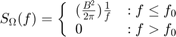
ここで、
B = バイアス不安定性係数
 = カットオフ周波数
元の PSD の方程式に代入して積分を実行すると、次のようになります。
![$$\sigma^2(\tau) = \frac{2B^2}{\pi}[\ln{2} + \\ -\frac{sin^3x}{2x^2}(sinx + 4xcosx) + Ci(2x) - Ci(4x)]$$](../../examples/shared_positioning/win64/AllanVarianceExample_eq05741459843801261458.png)
ここで、

Ci = 余弦積分関数
がカットオフ周波数の逆数よりもはるかに長い場合、PSD の方程式は次のようになります。
上記の方程式を と の両対数プロットでプロットすると、傾きが 0 の直線になります。この直線から  のスケーリングによって "B" の値を直接読み取ることができます。"B" の単位は
  です。
です。
% Find the index where the slope of the log-scaled Allan deviation is equal
% to the slope specified.
slope = 0;
logtau = log10(tau);
logadev = log10(adev);
dlogadev = diff(logadev) ./ diff(logtau);
[~, i] = min(abs(dlogadev - slope));

% Find the y-intercept of the line.
b = logadev(i) - slope*logtau(i);

% Determine the bias instability coefficient from the line.
scfB = sqrt(2*log(2)/pi);
logB = b - log10(scfB);
B = 10^logB

% Plot the results.
tauB = tau(i);
lineB = B * scfB * ones(size(tau));
figure
loglog(tau, adev, tau, lineB, '--', tauB, scfB*B, 'o')
title('Allan Deviation with Bias Instability')
xlabel('\tau')
ylabel('\sigma(\tau)')
legend('\sigma', '\sigma_B')
text(tauB, scfB*B, '0.664B')
grid on
axis equal
B =

    0.0020

すべてのノイズ パラメーターを計算したので、パラメーターの定量化に使用したすべての直線と一緒にアラン偏差をプロットします。
tauParams = [tauN, tauK, tauB];
params = [N, K, scfB*B];
figure
loglog(tau, adev, tau, [lineN, lineK, lineB], '--', ...
    tauParams, params, 'o')
title('Allan Deviation with Noise Parameters')
xlabel('\tau')
ylabel('\sigma(\tau)')
legend('$\sigma (rad/s)$', '$\sigma_N ((rad/s)/\sqrt{Hz})$', ...
    '$\sigma_K ((rad/s)\sqrt{Hz})$', '$\sigma_B (rad/s)$', 'Interpreter', 'latex')
text(tauParams, params, {'N', 'K', '0.664B'})
grid on
axis equal

ジャイロスコープのシミュレーション
imuSensor オブジェクトを使用して、上記で特定されたノイズ パラメーターを使ってジャイロスコープの測定をシミュレートします。
% Simulating the gyroscope measurements takes some time. To avoid this, the
% measurements were generated and saved to a MAT-file. By default, this
% example uses the MAT-file. To generate the measurements instead, change
% this logical variable to true.
generateSimulatedData = false;

if generateSimulatedData
    % Set the gyroscope parameters to the noise parameters determined
    % above. Use single-sided noise to match the parameter scaling and 500
    % poles for the bias instability model to match the hardware output.
    numpoles = 500;
    gyro = gyroparams('NoiseDensity', N, 'RandomWalk', K, ...
        'BiasInstability', B, 'NoiseType', 'single-sided', ...
        'BiasInstabilityCoefficients', fractalcoef(numpoles));
    omegaSim = helperAllanVarianceExample(L, Fs, gyro);
else
    load('SimulatedSingleAxisGyroscope', 'omegaSim')
end
シミュレートされるアラン偏差を計算し、ログ データと比較します。
[avarSim, tauSim] = allanvar(omegaSim, 'octave', Fs);
adevSim = sqrt(avarSim);
adevSim = mean(adevSim, 2); % Use the mean of the simulations.

figure
loglog(tau, adev, tauSim, adevSim, '--')
title('Allan Deviation of HW and Simulation')
xlabel('\tau');
ylabel('\sigma(\tau)')
legend('HW', 'SIM')
grid on
axis equal

プロットは、imuSensor から作成されたジャイロスコープ モデルで生成される測定について、アラン偏差がログ データと同程度になることを示しています。量子化パラメーターと温度関連パラメーターが gyroparams を使用して設定されていないため、モデルの測定の方がノイズがやや少なくなります。このジャイロスコープ モデルを使用して、ハードウェアでは簡単にキャプチャできない動きを使った測定値を生成できます。
参考文献
IEEE Std. 647-2006 IEEE Standard Specification Format Guide and Test Procedure for Single-Axis Laser Gyros