Main Content

simByEuler

Euler simulation of stochastic differential equations (SDEs) for SDE, BM, GBM, CEV, CIR, HWV, Heston, SDEDDO, SDELD, or SDEMRD models

Description

example

[Paths,Times,Z] = simByEuler(MDL,NPeriods) simulates NTrials sample paths of NVars correlated state variables driven by NBrowns Brownian motion sources of risk over NPeriods consecutive observation periods. simByEuler uses the Euler approach to approximate continuous-time stochastic processes.

example

[Paths,Times,Z] = simByEuler(___,Name,Value) specifies options using one or more name-value pair arguments in addition to the input arguments in the previous syntax.

You can perform quasi-Monte Carlo simulations using the name-value arguments for MonteCarloMethod, QuasiSequence, and BrownianMotionMethod. For more information, see Quasi-Monte Carlo Simulation.

Examples

collapse all

Load the Data and Specify the SDE Model

load Data_GlobalIdx2
prices  = [Dataset.TSX Dataset.CAC Dataset.DAX ...
    Dataset.NIK Dataset.FTSE Dataset.SP];

returns =  tick2ret(prices);

nVariables  = size(returns,2);
expReturn   = mean(returns);
sigma       = std(returns);
correlation = corrcoef(returns);
t           = 0;
X           = 100;
X           = X(ones(nVariables,1));

F = @(t,X) diag(expReturn)* X;
G = @(t,X) diag(X) * diag(sigma);

SDE = sde(F, G, 'Correlation', ...
    correlation, 'StartState', X);

Simulate a Single Path Over a Year

nPeriods = 249;      % # of simulated observations
dt       =   1;      % time increment = 1 day
rng(142857,'twister')
[S,T] = simByEuler(SDE, nPeriods, 'DeltaTime', dt);

Simulate 10 trials and examine the SDE model

rng(142857,'twister')
[S,T] = simulate(SDE, nPeriods, 'DeltaTime', dt, 'nTrials', 10);

whos S
  Name        Size               Bytes  Class     Attributes

  S         250x6x10            120000  double              
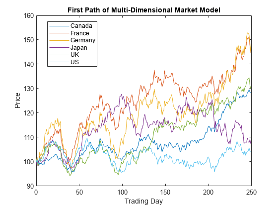
Plot the paths

plot(T, S(:,:,1)), xlabel('Trading Day'), ylabel('Price')
title('First Path of Multi-Dimensional Market Model')
legend({'Canada' 'France' 'Germany' 'Japan' 'UK' 'US'},...
    'Location', 'Best')

The Cox-Ingersoll-Ross (CIR) short rate class derives directly from SDE with mean-reverting drift (SDEMRD): dXt=S(t)[L(t)-Xt]dt+D(t,Xt12)V(t)dW

where D is a diagonal matrix whose elements are the square root of the corresponding element of the state vector.

Create a cir object to represent the model: dXt=0.2(0.1-Xt)dt+0.05Xt12dW.

CIR = cir(0.2, 0.1, 0.05)  % (Speed, Level, Sigma)
CIR = 
   Class CIR: Cox-Ingersoll-Ross
   ----------------------------------------
     Dimensions: State = 1, Brownian = 1
   ----------------------------------------
      StartTime: 0
     StartState: 1
    Correlation: 1
          Drift: drift rate function F(t,X(t)) 
      Diffusion: diffusion rate function G(t,X(t)) 
     Simulation: simulation method/function simByEuler
          Sigma: 0.05
          Level: 0.1
          Speed: 0.2

Simulate a single path over a year using simByEuler.

nPeriods = 249;      % # of simulated observations
dt       =   1;      % time increment = 1 day
rng(142857,'twister')
[Paths,Times] = simByEuler(CIR,nPeriods,'Method','higham-mao','DeltaTime', dt)
Paths = 250×1

    1.0000
    0.8613
    0.7245
    0.6349
    0.4741
    0.3853
    0.3374
    0.2549
    0.1859
    0.1814
      ⋮

Times = 250×1

     0
     1
     2
     3
     4
     5
     6
     7
     8
     9
      ⋮

The Cox-Ingersoll-Ross (CIR) short rate class derives directly from SDE with mean-reverting drift (SDEMRD): dXt=S(t)[L(t)-Xt]dt+D(t,Xt12)V(t)dW

where D is a diagonal matrix whose elements are the square root of the corresponding element of the state vector.

Create a cir object to represent the model: dXt=0.2(0.1-Xt)dt+0.05Xt12dW.

cir_obj = cir(0.2, 0.1, 0.05)  % (Speed, Level, Sigma)
cir_obj = 
   Class CIR: Cox-Ingersoll-Ross
   ----------------------------------------
     Dimensions: State = 1, Brownian = 1
   ----------------------------------------
      StartTime: 0
     StartState: 1
    Correlation: 1
          Drift: drift rate function F(t,X(t)) 
      Diffusion: diffusion rate function G(t,X(t)) 
     Simulation: simulation method/function simByEuler
          Sigma: 0.05
          Level: 0.1
          Speed: 0.2

Define the quasi-Monte Carlo simulation using the optional name-value arguments for 'MonteCarloMethod','QuasiSequence', and 'BrownianMotionMethod'.

[paths,time,z] = simByEuler(cir_obj,10,'ntrials',4096,'method','basic','montecarlomethod','quasi','quasisequence','sobol','BrownianMotionMethod','brownian-bridge');

The Heston (heston) class derives directly from SDE from Drift and Diffusion (sdeddo). Each Heston model is a bivariate composite model, consisting of two coupled univariate models:

dX1t=B(t)X1tdt+X2tX1tdW1t

dX2t=S(t)[L(t)-X2t]dt+V(t)X2tdW2t

Create a heston object.

heston_obj = heston (0.1, 0.2, 0.1, 0.05)  % (Return, Speed, Level, Volatility)
heston_obj = 
   Class HESTON: Heston Bivariate Stochastic Volatility
   ----------------------------------------------------
     Dimensions: State = 2, Brownian = 2
   ----------------------------------------------------
      StartTime: 0
     StartState: 1 (2x1 double array) 
    Correlation: 2x2 diagonal double array 
          Drift: drift rate function F(t,X(t)) 
      Diffusion: diffusion rate function G(t,X(t)) 
     Simulation: simulation method/function simByEuler
         Return: 0.1
          Speed: 0.2
          Level: 0.1
     Volatility: 0.05

Define the quasi-Monte Carlo simulation using the optional name-value arguments for 'MonteCarloMethod','QuasiSequence', and 'BrownianMotionMethod'.

[paths,time,z] = simByEuler(heston_obj,10,'ntrials',4096,'montecarlomethod','quasi','quasisequence','sobol','BrownianMotionMethod','principal-components');

Create a univariate gbm object to represent the model: dXt=0.25Xtdt+0.3XtdWt.

gbm_obj = gbm(0.25, 0.3)  % (B = Return, Sigma)
gbm_obj = 
   Class GBM: Generalized Geometric Brownian Motion
   ------------------------------------------------
     Dimensions: State = 1, Brownian = 1
   ------------------------------------------------
      StartTime: 0
     StartState: 1
    Correlation: 1
          Drift: drift rate function F(t,X(t)) 
      Diffusion: diffusion rate function G(t,X(t)) 
     Simulation: simulation method/function simByEuler
         Return: 0.25
          Sigma: 0.3

gbm objects display the parameter B as the more familiar Return.

Define the quasi-Monte Carlo simulation using the optional name-value arguments for 'MonteCarloMethod','QuasiSequence', and 'BrownianMotionMethod'.

[paths,time,z] = simByEuler(gbm_obj,10,'ntrials',4096,'montecarlomethod','quasi','quasisequence','sobol','BrownianMotionMethod','brownian-bridge');

Input Arguments

collapse all

Stochastic differential equation model, specified as an sde, bm, gbm, cev, cir, hwv, heston, sdeddo, sdeld, or sdemrd object.

Data Types: object

Number of simulation periods, specified as a positive scalar integer. The value of NPeriods determines the number of rows of the simulated output series.

Data Types: double

Name-Value Arguments

Specify optional pairs of arguments as Name1=Value1,...,NameN=ValueN, where Name is the argument name and Value is the corresponding value. Name-value arguments must appear after other arguments, but the order of the pairs does not matter.

Before R2021a, use commas to separate each name and value, and enclose Name in quotes.

Example: [Paths,Times,Z] = simByEuler(SDE,NPeriods,'DeltaTime',dt)

Method to handle negative values, specified as the comma-separated pair consisting of 'Method' and a character vector or string with a supported value.

Note

The Method argument is only supported when using a CIR object. For more information on creating a CIR object, see cir.

Data Types: char | string

Simulated trials (sample paths) of NPeriods observations each, specified as the comma-separated pair consisting of 'NTrials' and a positive scalar integer.

Data Types: double

Positive time increments between observations, specified as the comma-separated pair consisting of 'DeltaTime' and a scalar or a NPeriods-by-1 column vector.

DeltaTime represents the familiar dt found in stochastic differential equations, and determines the times at which the simulated paths of the output state variables are reported.

Data Types: double

Number of intermediate time steps within each time increment dt (specified as DeltaTime), specified as the comma-separated pair consisting of 'NSteps' and a positive scalar integer.

The simByEuler function partitions each time increment dt into NSteps subintervals of length dt/NSteps, and refines the simulation by evaluating the simulated state vector at NSteps − 1 intermediate points. Although simByEuler does not report the output state vector at these intermediate points, the refinement improves accuracy by allowing the simulation to more closely approximate the underlying continuous-time process.

Data Types: double

Flag that indicates whether simByEuler uses antithetic sampling to generate the Gaussian random variates that drive the Brownian motion vector (Wiener processes). This argument is specified as the comma-separated pair consisting of 'Antithetic' and a scalar logical flag with a value of True or False.

When you specify True, simByEuler performs sampling such that all primary and antithetic paths are simulated and stored in successive matching pairs:

  • Odd trials (1,3,5,...) correspond to the primary Gaussian paths.

  • Even trials (2,4,6,...) are the matching antithetic paths of each pair derived by negating the Gaussian draws of the corresponding primary (odd) trial.

Note

If you specify an input noise process (see Z), simByEuler ignores the value of Antithetic.

Data Types: logical

Direct specification of the dependent random noise process used to generate the Brownian motion vector (Wiener process) that drives the simulation. This argument is specified as the comma-separated pair consisting of 'Z' and a function or as an (NPeriods ⨉ NSteps)-by-NBrowns-by-NTrials three-dimensional array of dependent random variates.

Note

If you specify Z as a function, it must return an NBrowns-by-1 column vector, and you must call it with two inputs:

  • A real-valued scalar observation time t.

  • An NVars-by-1 state vector Xt.

Data Types: double | function

Flag that indicates how the output array Paths is stored and returned, specified as the comma-separated pair consisting of 'StorePaths' and a scalar logical flag with a value of True or False.

  • If StorePaths is True (the default value) or is unspecified, simByEuler returns Paths as a three-dimensional time series array.

  • If StorePaths is False (logical 0), simByEuler returns the Paths output array as an empty matrix.

Data Types: logical

Monte Carlo method to simulate stochastic processes, specified as the comma-separated pair consisting of 'MonteCarloMethod' and a string or character vector with one of the following values:

  • "standard" — Monte Carlo using pseudo random numbers

  • "quasi" — Quasi-Monte Carlo using low-discrepancy sequences

  • "randomized-quasi" — Randomized quasi-Monte Carlo

Note

If you specify an input noise process (see Z), simByEuler ignores the value of MonteCarloMethod.

Data Types: string | char

Low discrepancy sequence to drive the stochastic processes, specified as the comma-separated pair consisting of 'QuasiSequence' and a string or character vector with the following value:

  • "sobol" — Quasi-random low-discrepancy sequences that use a base of two to form successively finer uniform partitions of the unit interval and then reorder the coordinates in each dimension.

Note

If MonteCarloMethod option is not specified or specified as"standard", QuasiSequence is ignored.

Data Types: string | char

Brownian motion construction method, specified as the comma-separated pair consisting of 'BrownianMotionMethod' and a string or character vector with one of the following values:

  • "standard" — The Brownian motion path is found by taking the cumulative sum of the Gaussian variates.

  • "brownian-bridge" — The last step of the Brownian motion path is calculated first, followed by any order between steps until all steps have been determined.

  • "principal-components" — The Brownian motion path is calculated by minimizing the approximation error.

Note

If an input noise process is specified using the Z input argument, BrownianMotionMethod is ignored.

The starting point for a Monte Carlo simulation is the construction of a Brownian motion sample path (or Wiener path). Such paths are built from a set of independent Gaussian variates, using either standard discretization, Brownian-bridge construction, or principal components construction.

Both standard discretization and Brownian-bridge construction share the same variance and, therefore, the same resulting convergence when used with the MonteCarloMethod using pseudo random numbers. However, the performance differs between the two when the MonteCarloMethod option "quasi" is introduced, with faster convergence for the "brownian-bridge" construction option and the fastest convergence for the "principal-components" construction option.

Data Types: string | char

Sequence of end-of-period processes or state vector adjustments of the form, specified as the comma-separated pair consisting of 'Processes' and a function or cell array of functions of the form

Xt=P(t,Xt)

The simByEuler function runs processing functions at each interpolation time. They must accept the current interpolation time t, and the current state vector Xt, and return a state vector that may be an adjustment to the input state.

If you specify more than one processing function, simByEuler invokes the functions in the order in which they appear in the cell array. You can use this argument to specify boundary conditions, prevent negative prices, accumulate statistics, and plot graphs.

Data Types: cell | function

Output Arguments

collapse all

Simulated paths of correlated state variables, returned as an (NPeriods + 1)-by-NVars-by-NTrials three-dimensional time series array.

For a given trial, each row of Paths is the transpose of the state vector Xt at time t. When the input flag StorePaths = False, simByEuler returns Paths as an empty matrix.

Observation times associated with the simulated paths, returned as an (NPeriods + 1)-by-1 column vector. Each element of Times is associated with the corresponding row of Paths.

Dependent random variates used to generate the Brownian motion vector (Wiener processes) that drive the simulation, returned as an (NPeriods ⨉ NSteps)-by-NBrowns-by-NTrials three-dimensional time series array.

More About

collapse all

Antithetic Sampling

Simulation methods allow you to specify a popular variance reduction technique called antithetic sampling.

This technique attempts to replace one sequence of random observations with another of the same expected value, but smaller variance. In a typical Monte Carlo simulation, each sample path is independent and represents an independent trial. However, antithetic sampling generates sample paths in pairs. The first path of the pair is referred to as the primary path, and the second as the antithetic path. Any given pair is independent of any other pair, but the two paths within each pair are highly correlated. Antithetic sampling literature often recommends averaging the discounted payoffs of each pair, effectively halving the number of Monte Carlo trials.

This technique attempts to reduce variance by inducing negative dependence between paired input samples, ideally resulting in negative dependence between paired output samples. The greater the extent of negative dependence, the more effective antithetic sampling is.

Algorithms

This function simulates any vector-valued SDE of the form

dXt=F(t,Xt)dt+G(t,Xt)dWt

where:

  • X is an NVars-by-1 state vector of process variables (for example, short rates or equity prices) to simulate.

  • W is an NBrowns-by-1 Brownian motion vector.

  • F is an NVars-by-1 vector-valued drift-rate function.

  • G is an NVars-by-NBrowns matrix-valued diffusion-rate function.

simByEuler simulates NTrials sample paths of NVars correlated state variables driven by NBrowns Brownian motion sources of risk over NPeriods consecutive observation periods, using the Euler approach to approximate continuous-time stochastic processes.

  • This simulation engine provides a discrete-time approximation of the underlying generalized continuous-time process. The simulation is derived directly from the stochastic differential equation of motion. Thus, the discrete-time process approaches the true continuous-time process only as DeltaTime approaches zero.

  • The input argument Z allows you to directly specify the noise-generation process. This process takes precedence over the Correlation parameter of the sde object and the value of the Antithetic input flag. If you do not specify a value for Z, simByEuler generates correlated Gaussian variates, with or without antithetic sampling as requested.

  • The end-of-period Processes argument allows you to terminate a given trial early. At the end of each time step, simByEuler tests the state vector Xt for an all-NaN condition. Thus, to signal an early termination of a given trial, all elements of the state vector Xt must be NaN. This test enables a user-defined Processes function to signal early termination of a trial, and offers significant performance benefits in some situations (for example, pricing down-and-out barrier options).

References

[1] Deelstra, G. and F. Delbaen. “Convergence of Discretized Stochastic (Interest Rate) Processes with Stochastic Drift Term.” Applied Stochastic Models and Data Analysis, 1998, Vol. 14, No. 1, pp. 77–84.

[2] Higham, Desmond, and Xuerong Mao. “Convergence of Monte Carlo Simulations Involving the Mean-Reverting Square Root Process.” The Journal of Computational Finance, Vol. 8, No. 3, 2005, pp. 35–61.

[3] Lord, Roger, et al. “A Comparison of Biased Simulation Schemes for Stochastic Volatility Models.” Quantitative Finance, Vol. 10, No. 2, Feb. 2010, pp. 177–94

Version History

Introduced in R2008a

expand all