Model Local Trends in Global Carbon Emissions

Global carbon emissions have increased dramatically in the last century. However, the annual growth rates are time-varying and have moderated in recent years, possibly due to international efforts on climate change under the Kyoto Protocol (1997), the Paris Agreement (2015), and exogenous shocks during the COVID-19 pandemic (2020 onward).

This example analyzes time-varying local trends in carbon emissions data by building dynamic state-space models from series for coal, gas, and oil. A useful feature of the state-space model is that you can incorporate unobserved components, such as local trends, into the state variables.

Specify Local Trend Model

Load the Data_CarbonEmissions.mat data set, provided by Haver Analytics®, which contains historical annual carbon emissions measurements from coal, gas, and oil combustion.

load Data_CarbonEmissions

coal = Data(:,1);   
gas = Data(:,2);    
oil = Data(:,3);    
total = Data(:,4);  % Total emissions from coal, gas, oil, and other industries (e.g., cement, flaring)

Plot the series in the same figure.

plot(dates,Data)
xlabel("Year");
ylabel("Emissions (Billions of Metric Tons)");
title("Global Carbon Emissions")
legend(["Coal" "Gas" "Oil" "Total"],Location="northwest")
axis tight
grid on

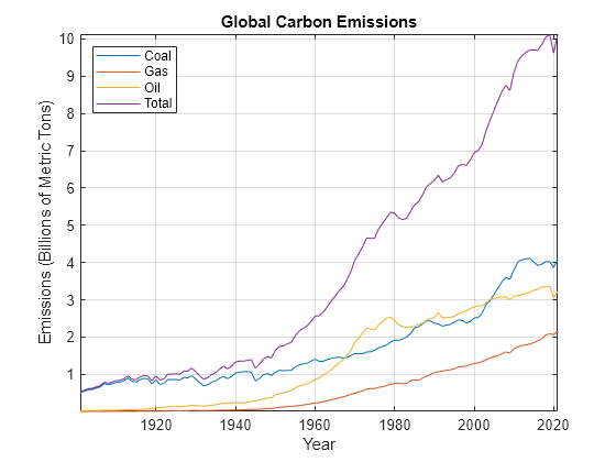
The time series plots show that carbon emissions have been increasing at overall increasing rates. A single, deterministic linear trend provides a poor description. Local trend models better capture the time-varying growth pattern.

Let ${\tau }_t$ be a local trend for which the first difference $\mathrm{\Delta }{\tau }_t={\tau }_t-{\tau }_{t-1}$ follows a random walk process,

$$\mathrm{\Delta }{\tau }_t=\mathrm{\Delta }{\tau }_{t-1}+{\sigma }_u{u}_t,$$

where $u_t$ is a series of standard normal innovations. The trend model has intercept ${\tau }_0$ and initial slope $\mathrm{\Delta }{\tau }_0$.

Suppose that the observations in the emissions data ${\mathit{y}}_t$ are noisy measurements of the local trend,

$${\mathit{y}}_t={\tau }_t+{\sigma }_{\epsilon }{\epsilon }_t,$$

where ${\epsilon }_t$ is another series of standard normal innovations.

This state-space model captures the combined effects.

$$\left(\begin{array}{c}{\tau }_t\\ {\tau }_{t-1}\end{array}\right)=\left(\begin{array}{cc}2& -1\\ 1& 0\end{array}\right)\left(\begin{array}{c}{\tau }_{t-1}\\ {\tau }_{t-2}\end{array}\right)+\left(\begin{array}{c}{\sigma }_u\\ 0\end{array}\right)u_t$$

$${\mathit{y}}_t=\left(\begin{array}{cc}1& 0\end{array}\right)\left(\begin{array}{c}{\tau }_t\\ {\tau }_{t-1}\end{array}\right)+{\sigma }_{\epsilon }{\epsilon }_t.$$

The paramMap function in the Supporting Functions section evaluates this model at an input vector of the parameters.

Estimate and Forecast Local Trend Model

Econometrics Toolbox™ supports a variety of state-space models. The ssm object represents a linear Gaussian state-space model.

Create a linear Gaussian state-space model by passing the parameter mapping function paramMap that specifies the local trend model. Then, apply maximum likelihood to estimate the unknown parameters. This example fits the model to the total carbon emissions series; you can use the drop-down list control to choose a different series.

Mdl = ssm(@paramMap);     
Y = total; 
params0 = [0.1;0.1;0.5;0.01];
EstMdl = estimate(Mdl,Y,params0,Univariate=true,LB=zeros(4,1));

Method: Maximum likelihood (fmincon)
Sample size: 121
Logarithmic  likelihood:      70.8188
Akaike   info criterion:     -133.638
Bayesian info criterion:     -122.454
      |     Coeff        Std Err     t Stat     Prob  
------------------------------------------------------
 c(1) |  0.03940         0.00496     7.95246   0      
 c(2) |  0.08036         0.00392    20.50197   0      
 c(3) |  0.51510       112.36483     0.00458  0.99634 
 c(4) |  0.02901         0.53690     0.05403  0.95691 
      |                                               
      |   Final State     Std Dev     t Stat    Prob  
 x(1) | 10.00230         0.06406   156.13238   0      
 x(2) |  9.96228         0.04541   219.40803   0      

Based on the fitted model, the Kalman filter and smoother provide state estimation. The first state variable is the local trend estimate.

States = smooth(EstMdl,Y);
localTrend = States(:,1);

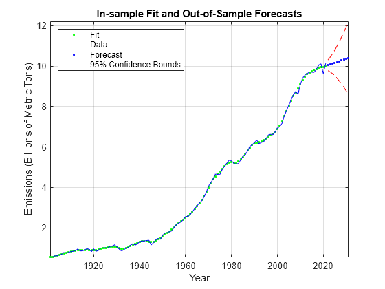
The estimated local trend facilitates out-of-sample forecasting. Without new observations, assume that the current state of growth momentum passes on to the forecast periods. The Kalman filter provides the forecast carbon emission levels.

Forecast the local trend model and compute approximate 95% forecast intervals. Plot the forecasts and intervals with the data. This example uses a forecast horizon of 10 years; you can use the slider control to adjust the horizon.

n = 10; 
[yf,yfMSE] = forecast(EstMdl,n,Y);
yfLB = yf - 2*sqrt(yfMSE); % Lower 95% confidence bound
yfUB = yf + 2*sqrt(yfMSE); % Upper 95% confidence bound
xf = (dates(end)+1:dates(end)+n)'; % Forecast horizon

plot(dates,localTrend,".g",dates,Y,"-b",xf,yf,".b", ...
    xf,yfLB,"--r",xf,yfUB,"--r");
xlabel("Year");
ylabel("Emissions (Billions of Metric Tons)");
title("In-sample Fit and Out-of-Sample Forecasts")
legend(["Fit" "Data" "Forecast" "95% Confidence Bounds"],Location="northwest")
axis tight
grid on

Include Intervention Effects Using Dummy Variables

Intervention terms in the model can measure the effects of the Kyoto Protocol and Paris Agreement on carbon emissions, as countries work towards carbon neutrality. Also, an intervention term in the model can measure whether exogenous shocks from the COVID-19 pandemic, which slowed down the world economy, also impacted emissions.

Create dummy variables to indicate these interventions on the climate.

kyoto = dates > 1997;
paris = dates > 2015;
covid = dates >= 2020;
Dummy = [kyoto paris covid];
nvar = size(Dummy,2);

Add exogenous predictors to the observation equation of the state-space model. The paramMapDummy function in the Supporting Functions section evaluates this model at an input vector of the parameters.

MdlDummy = ssm(@(params)paramMapDummy(params,total,Dummy));

Fit the model to the data.

params0Dummy = [params0; zeros(nvar,1)];
[~,estParams] = estimate(MdlDummy,total,params0Dummy, ...
    Univariate=true,LB=[zeros(4,1); -Inf(nvar,1)]);

Method: Maximum likelihood (fmincon)
Sample size: 121
Logarithmic  likelihood:      86.6833
Akaike   info criterion:     -159.367
Bayesian info criterion:     -139.796
      |     Coeff        Std Err     t Stat     Prob  
------------------------------------------------------
 c(1) |  0.05776         0.00607     9.51503   0      
 c(2) |  0.05491         0.00372    14.77908   0      
 c(3) |  0.52101       190.70633     0.00273  0.99782 
 c(4) |  0.02587         0.88069     0.02938  0.97656 
 c(5) | -0.17006         0.32437    -0.52430  0.60007 
 c(6) | -0.13309         0.15597    -0.85329  0.39350 
 c(7) | -0.74058         0.10635    -6.96347   0      
      |                                               
      |   Final State     Std Dev     t Stat    Prob  
 x(1) | 11.09826         0.04843   229.14712   0      
 x(2) | 10.74580         0.03551   302.64372   0      

The last three coefficients c(5) through c(7) correspond to the intervention variables. Results show a significant negative effect on emissions.

disp(estParams(5:7)')

   -0.1701   -0.1331   -0.7406

Analyze Multivariate Model with Common Stochastic Trend

An alternative approach to the univariate model assumes that a common stochastic trend drives global carbon emissions from all sources. This model is a dynamic factor model, in which the common local trend is an unobserved factor underlying all observed time series.

First, reparametrize the local trend as

${\tilde{\tau }}_t={\sigma }_u^{-1}\left({\tau }_t-{\tau }_0-\mathrm{\Delta }{\tau }_{0}t\right).$

The reparametrized state-space model without intervention effects is

$\left(\begin{array}{c}{\tilde{\tau }}_t\\ {\tilde{\tau }}_{t-1}\end{array}\right)=\left(\begin{array}{cc}2& -1\\ 1& 0\end{array}\right)\left(\begin{array}{c}{\tilde{\tau }}_{t-1}\\ {\tilde{\tau }}_{t-2}\end{array}\right)+\left(\begin{array}{c}1\\ 0\end{array}\right)u_t,$

$${\mathit{y}}_t={\tau }_0+\mathrm{\Delta }{\tau }_{0}t+\left(\begin{array}{cc}{\sigma }_u& 0\end{array}\right)\left(\begin{array}{c}{\tilde{\tau }}_t\\ {\tilde{\tau }}_{t-1}\end{array}\right)+{\sigma }_{\epsilon }{\epsilon }_t.$$

The reparametrized model facilitates multivariate extension, in which each series has its own parameters ${\sigma }_u$, ${\sigma }_{\epsilon }$, ${\tau }_0$ and $\mathrm{\Delta }{\tau }_0$, while all series are determined by the common normalized local trend. The paramMapFactor function in the Supporting Functions section evaluates this model at an input vector of the parameters.

In the year 1901, global carbon emissions from gas and oil were close to zero. Assume that ${\tau }_0$ and $\mathrm{\Delta }{\tau }_0$ are zero to simplify parameter estimation. Specify the multivariate model and apply maximum likelihood to estimate the unknown parameters.

Y = [coal gas oil];
MdlFactor = ssm(@(params)paramMapFactor(params,Y)); 
params0Factor = [0.1*ones(3,1); 0.1*ones(3,1); 0.5; 0.01];
estimate(MdlFactor,Y,params0Factor,Univariate=true, ...
    LB=zeros(size(params0Factor)));

Method: Maximum likelihood (fmincon)
Sample size: 121
Logarithmic  likelihood:      271.493
Akaike   info criterion:     -526.986
Bayesian info criterion:     -504.619
      |      Coeff       Std Err    t Stat     Prob  
-----------------------------------------------------
 c(1) |   0.00498       0.00076     6.54405   0      
 c(2) |   0.00334       0.00050     6.68119   0      
 c(3) |   0.00685       0.00103     6.66525   0      
 c(4) |   0.16843       0.01224    13.75782   0      
 c(5) |   0.01371       0.00061    22.46811   0      
 c(6) |   0.45913       0.03080    14.90797   0      
 c(7) |   0.73505       0.06506    11.29855   0      
 c(8) |   0.00205       0.00172     1.19255  0.23305 
      |                                              
      |    Final State   Std Dev     t Stat    Prob  
 x(1) | 643.03746       2.89879   221.82971   0      
 x(2) | 629.50544       2.15224   292.48818   0      

Local trend models capture time-varying behavior and provide a good fit for the global carbon emissions data.

Supporting Functions

Each function in this section specifies the state-space model structure of the corresponding model in this example.

function [A,B,C,D,mean0,Cov0] = paramMap(params)
sigmaU = params(1);
sigmaE = params(2);
intercept = params(3);
slope = params(4);
A = [2 -1; 1 0];
B = [sigmaU; 0];
C = [1 0];
D = sigmaE;
mean0 = [intercept; intercept - slope];
Cov0 = ones(2);
end

function [A,B,C,D,mean0,Cov0,stateType,yDeflate] = paramMapDummy(params,y,Dummy)
sigmaU = params(1);
sigmaE = params(2);
intercept = params(3);
slope = params(4);
dummyCoeff = params(5:end);
A = [2 -1; 1 0];
B = [sigmaU; 0];
C = [1 0];
D = sigmaE;
mean0 = [intercept; intercept-slope];
Cov0 = ones(2);
stateType = [2; 2];
yDeflate = y - Dummy*dummyCoeff;
end

function [A,B,C,D,mean0,Cov0,stateType,YDeflate] = paramMapFactor(params,Y)
sigmaU = params(1:3);
sigmaE = params(4:6);
intercept = params(7);
slope = params(8);
A = [2 -1; 1 0];
B = [1; 0];
C = [sigmaU, zeros(3,1)];
D = diag(sigmaE);
mean0 = [0; 0];
Cov0 = ones(2);
stateType = [2; 2];
linear = [intercept; 0; 0] + [slope; 0; 0] .* (1:size(Y,1));
YDeflate = Y - linear';
end

References

[1] "The Global Carbon Project", accessed November 11, 2023, https://www.globalcarbonproject.org.