Model and Forecast Business Cycles Using Econometric Modeler App

This example shows how to use Econometric Modeler to decompose a time series into long- and short-term components, which you can use to study business cycles. The time series is the quarterly US gross domestic product (GDP), measured 1947 through 2005.

Economic time series can be viewed as the sum of long-term trends and short-term fluctuations. The short-term fluctuations, as called business cycles, are of particular interest because they can indicate periods of economic expansion, contraction, or stagnation. The Econometric Modeler app enables you to decompose economic time series into the long- and short-term components by applying several data filters. This example uses the Baxter-King filter [1]; for choosing a data filter for your data, see Choose Time Series Filter for Business Cycle Analysis.

At the command line, load the Data_GDP.mat data set.

load Data_GDP

DataTimeTable is a timetable containing time series data.

At the command line, open the Econometric Modeler app.

econometricModeler

Alternatively, open the app from the apps gallery (see Econometric Modeler).

Import DataTimeTable into the app:

1. On the Modeler tab, in the Import section, click the Import button .

2. In the Import Data dialog box, select the check box for the DataTimeTable variable.

3. Click Import.

The variable GDP appears in the Time Series pane, and its time series plot is in the Plot(GDP) figure window.

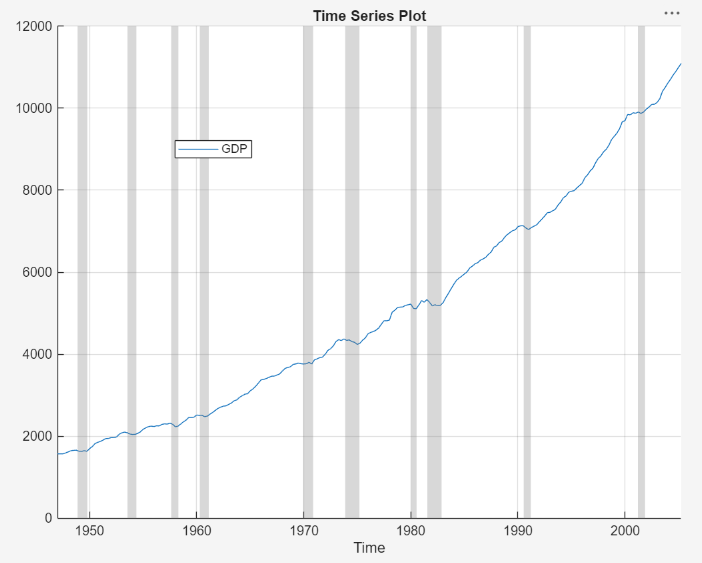
The time series drifts upward with a clear cyclical component around the trend.

Apply the Baxter-King filter to the time series. On the Modeler tab, in the Filters section, click Filter Data > Baxter-King Filter. The Baxter-King Filter dialog appears containing parameter settings and a plot of the time series and trend component at the current parameter settings.

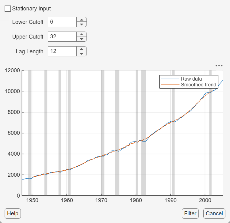
Arbitrarily adjust the lower and upper cutoff, and lag length, parameters to see how the adjustments change the trend. The trend's shape immediately changes as you adjust the settings. Observe that the trend follows the time series more closely as you decrease the lag length or cutoff interval, and the trend smooths out as you increase either parameter.

Although you can apply rules of thumb to adjust the parameters, for example, for quarterly data, Baxter and King [1] suggest a lag length of 12 quarters, the goal is to find a balance between a trend that follows the peaks and valleys in the data and is smooth. A trend that follows the data too closely results in a cyclical component that is not informative, and a trend that is too smooth results in a cyclical component that might be too noisy to extract a business cycle.

Set the parameters to their default values, and in the figure, and click Filter. In the left panel, the GDP_BKCycle and GDP_BKTrend variables appear, which contain the cyclical and trend component time series, respectively, from applying the Baxter-King filter. In the right panel, a figure containing a time series plot of the cyclical (left y axis) and trend (right y-axis) components appears.

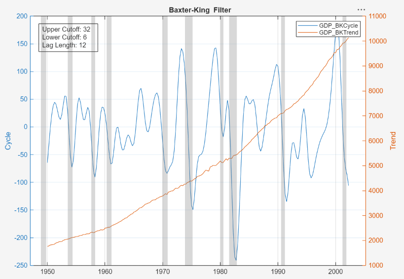
The trend component increases exponentially. The cyclical component shows peaks just before recession, and deep valleys during and just after recessions. This behavior suggests that the cyclical component might be a good description of the business cycle. Also, observe that the components have fewer observations than the GDP series. This happens because the filter requires Lag Length observations from the head and tail of the series.

Plot the ACF and PACF of the cyclical component. In the Modeler tab, in the Time Series pane, select the GDP_BKCycle variable. Then, in the Plots tab, in the Plots section, click ACF and then PACF. In the right pane, plots of the ACF and PACF of the GDP cyclical component appear in the ACF(GDP_BKCycle) and PACF(GDP_BKCycle) tabs, respectively. Arrange the ACF plot above the PACF plot.

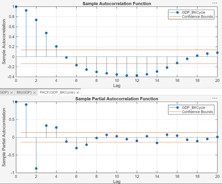
The ACF decays sinusoidally. The first insignificant lag of the PACF is at 5, but lags 6, 7 and some larger lags are significant. This behavior is indicative of an AR(p) model, where p ≥ 6.

For model parsimony, fit an AR(6) model to the GDP cyclical component time series.

1. In the Modeler tab, in the Models section, click AR.

2. In the AR Model Parameters dialog, set the Autoregressive Order (p) parameter to 6.

3. Click Estimate. In the right pane, an estimation summary appears. In the Time Series pane, in the Models section, the estimated model AR_GDP_BKCycle appears.

4. Close the partition between the documents and the PACF.

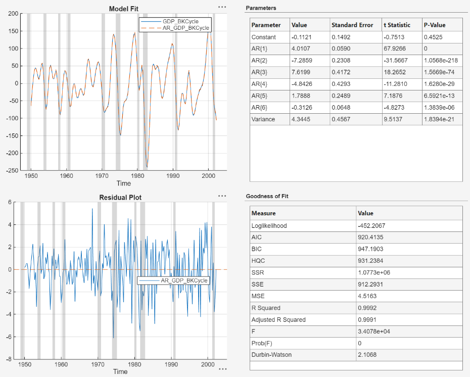
The model shows an tight in-sample fit; all coefficients except for the constant are significant. The residuals appear randomly spread, but might show some volatility clustering. The Durbin-Watson statistic is close to 2, which suggests little autocorrelation in the residual series. This example proceeds without addressing possible heteroscedasticity.

Forecast the GDP cyclical component into a 5-year (20-point for monthly data) horizon beyond the in-sample data, which is from Q3-2005 through Q2-2010.

1. In the Models pane, select AR_GDP_BKCycle.

2. In the Modeler tab, in the Forecast section, click Forecast.

3. In the Forecast Model Response dialog, set the Number of periods in forecast horizon parameter to 20.

4. Click Forecast.

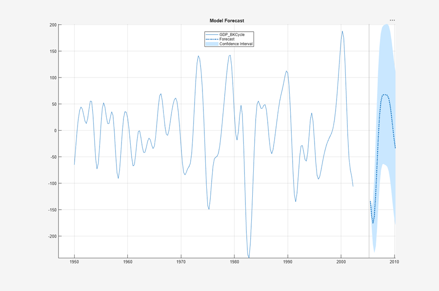
The forecasts suggest an expansion at the end of 2005, followed by an economic downturn starting around 2008. Observe that forecasts begin at the period after end of the timebase of the imported data, not the estimation sample of the model, which explains the gap in the series between around 2002 to the beginning of the forecast sample.

References

[1] Baxter, Marianne, and Robert G. King. "Measuring Business Cycles: Approximate Band-Pass Filters for Economic Time Series." Review of Economics and Statistics 81, no. 4 (November 1999): 575–93. https://doi.org/10.1162/003465399558454.