Choose Time Series Filter for Business Cycle Analysis

This example compares the performance of the Hodrick-Prescott filter (hpfilter) for business cycle analysis with the performance of alternatives in the context of various economic data-generating processes. The alternative business cycle filters, available with Econometrics Toolbox™, are the:

• Baxter-King filter [1], as computed by the bkfilter function

• Christiano-Fitzgerald filter [4], as computed by the cffilter function

• One-sided Hodrick-Prescott filter [15], as computed by the hpfilter function

• Hamilton filter [9], as computed by the hfilter function

This example uses historical data sets available with Econometrics Toolbox. For current data, download series from the Federal Reserve Economic Data (FRED) database on the Federal Reserve Bank of St. Louis website at https://fred.stlouisfed.org/.

What Is a Business Cycle?

The forces that shape a macroeconomy cause both long-term trends and temporary fluctuations in econometric data. Long-term secular influences include population growth, capital accumulation, productivity enhancements, and market development. Short-term influences include seasonality, regulatory intervention, central bank policies, technology shocks, and investor outlook. When observed in aggregate over multiple indicators of growth, medium-term variations in the economy are often described as recessions and expansions, or business cycles. Despite the suggestion of regularity, these empirical cycles are nondeterministic, aperiodic, and a mixture of frequencies.

Business cycles are evident in many macroeconomic time series. For example, the monthly US unemployment rate from 1954 through 1998 shows a distinctive pattern of peaks and troughs.

To see the business cycle, load the monthly US unemployment data Data_Unemployment.mat.

load Data_Unemployment

The variable Data is a 45-by-12 data matrix with months January through December as columns and years 1954 through 1998 as rows.

Arrange the data as one column vector of increasing observation times. Create a datetime vector of observation times.

Data = Data';
UN = Data(:);

tstart = datetime(dates(1),1,1);
tend = datetime(dates(end),12,1);
tUN = tstart:calmonths(1):tend;

Plot the series and overlay recession bands determined by the National Bureau of Economic Research (NBER).

figure
plot(tUN,UN)
recessionplot
ylabel("Rate (%)")
title("Unemployment Rate")

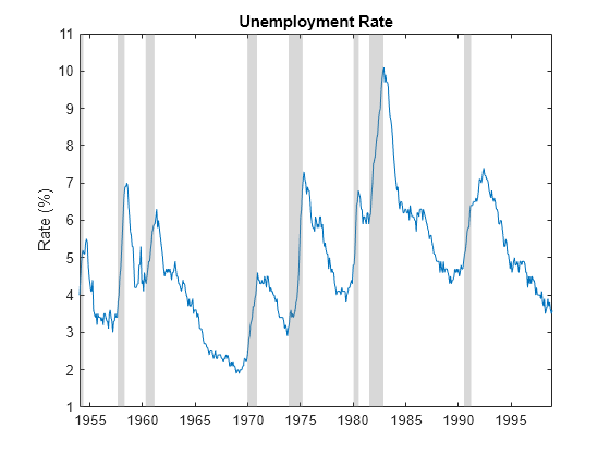
In such series, you can attempt to distinguish a trend component, accounting for long-term growth, and a cyclical component, capturing shorter-term deviations from the trend. What constitutes a trend and cycle, however, is a matter of problem formulation, analytic objectives, and the data available.

Methods for achieving trend-cycle decompositions of economic time series have a long history. Burns and Mitchell [3] were the first to describe the stylized facts of business cycles in the modern era. They defined US business cycles as cyclical components with a duration of no less than 6 quarters (18 months) and no more than 32 quarters (8 years). Their method requires the investigator's judgement to find peaks and troughs in empirical data, then compare them to reference cycles. The process is ill-suited to computer-driven analytics.

Hodrick-Prescott Filter

Hodrick and Prescott [11] sought to develop an analogue to the Burns and Mitchell approach with a clear computational basis.

The Hodrick-Prescott filter removes a low-frequency trend ${\tau }_{\mathit{t}}$ from a time series ${\mathit{y}}_{\mathit{t}}$ and assigns the remaining high-frequency components to a cycle ${\mathit{c}}_{\mathit{t}}$, so that ${\mathit{y}}_{\mathit{t}}={\tau }_{\mathit{t}}+{\mathit{c}}_{\mathit{t}}$. The filter identifies the components ${\tau }_{\mathit{t}}$ and ${\mathit{c}}_{\mathit{t}}$ by minimizing the objective function

$\sum _{\mathit{t}=1}^{\mathit{T}}{\mathit{c}}_{\mathit{t}}^2+\lambda \sum _{\mathit{t}=2}^{\mathit{T}-1}{\left(\left({\tau }_{\mathit{t}+1}-{\tau }_{\mathit{t}}\right)-\left({\tau }_{\mathit{t}}-{\tau }_{\mathit{t}-1}\right)\right)}^2$,

where $\mathit{T}$ is the sample size of ${\mathit{y}}_{\mathit{t}}$ and $\lambda$ is a tunable smoothing parameter. The first term minimizes the deviation of the cyclical component ${\mathit{c}}_{\mathit{t}}={\mathit{y}}_{\mathit{t}}-{\tau }_{\mathit{t}}$from the overall series data. The second term is a numerical second derivative of ${\tau }_{\mathit{t}}$, so that minimization penalizes rapid changes in the slope of the trend to a degree determined by $\lambda$. The derivative is centered at time $\mathit{t}$, incorporating past and future values, making the filter two-sided and noncausal.

The Hodrick-Prescott filter identifies the trend component through smoothing. The frequencies assigned to the cyclical component are highpass, and do not correspond to any specific definition of business cycle. Hodrick and Prescott say of the cyclical component that "the fluctuations studied are those that are too rapid to be accounted for by slowly changing demographic and technological factors and changes in stocks of capital that produce secular growth in output per capita."

The hpfilter function implements the Hodrick-Prescott filter. For monthly data such as the unemployment rate series, Hodrick and Prescott recommend a smoothing parameter of $\lambda$ = 14,400.

[UNHPTrend,UNHPCycle] = hpfilter(UN,Smoothing=14400);

Ravn and Uhlig [13] reassess the Hodrick-Prescott filter and recommend a more aggressive smoothing parameter for monthly data of $\lambda$ = 129,600.

[UNRUTrend,UNRUCycle] = hpfilter(UN,Smoothing=129600);

Visually compare the resulting trend components.

figure
hold on
plot(tUN,UN)
plot(tUN,UNHPTrend,"r")
plot(tUN,UNRUTrend,"m:",LineWidth=2)
recessionplot
hold off
ylabel("Rate (%)")
title("Unemployment Rate")
legend(["Data" "HP trend" "RU trend"])

Visually compare the resulting cyclical components, which are the difference between the data and the trends.

figure
hold on
plot(tUN,UNHPCycle,"r")
plot(tUN,UNRUCycle,"m:",LineWidth=2)
recessionplot
hold off
ylabel("Cyclical Component")
title("Unemployment Rate")
legend(["HP cycle" "RU cycle"])

Greater smoothing of the Ravn-Uhlig trend leads to larger absolute deviations in the cycle.

Baxter-King Filter

Granger [8] notes that the “typical spectral shape” of macroeconomic time series exhibits substantial power in a range of low frequencies, a high-frequency noise component from aggregated variables, and a business cycle in between.

The approach of Baxter and King [1] is focused on the specific definition of business cycle adopted by Burns and Mitchell: "Technically, we develop approximate band-pass filters that are constrained to produce stationary outcomes when applied to growing time series. For the empirical applications... we adopt the definition of business cycles suggested by the procedures and findings of NBER researchers like Burns and Mitchell." The band-pass methodology of Baxter and King formalizes Granger's insights and combines them with the conclusions of Burns and Mitchell, making rigorous a consensus perspective in macroeconomics.

The bkfilter function implements the Baxter-King filter. Because it is a bandpass filter, the function requires upper and lower cutoff periods (UpperCutoff and LowerCutoff name-value arguments), in units of data periodicity, to delineate the extent of the business cycle. Instead of a smoothing parameter, an optional lag-length parameter (LagLength name-value argument) adjusts the size of a symmetric, time-invariant moving average that smooths the data and extracts a trend component. The fixed lag length results in data trimming on both ends of the data.

Although this approach is different from that of Hodrick and Prescott, for many macroeconomic series, the Baxter-King filter produces similar results. To compare the results, load the US Gross Domestic Product (GDP) data set Data_GDP, which contains quarterly measurements of the US GDP from 1947 through 2005. Plot the series.

load Data_GDP
GDP = Data;
tGDP = datetime(dates,ConvertFrom="datenum");

figure
plot(tGDP,GDP)
recessionplot
ylabel("Billions of Dollars")
title("Gross Domestic Product")

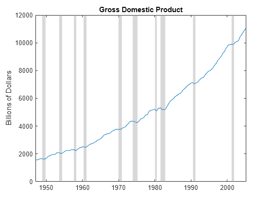
The data drifts upward with a clear cyclical component around the trend.

For quarterly data, Hodrick-Prescott and Ravn-Uhlig recommendations for the smoothing parameter coincide. Burns and Mitchell cutoffs for the bandpass filter are at 6 and 32 quarters. Baxter and King suggest a lag length of 12 quarters.

Apply the Hodrick-Prescott and Baxter-King filters to the US GDP series. Visually compare the cyclical components.

[~,GDPHPCycle] = hpfilter(GDP);
[~,GDPBKCycle] = bkfilter(GDP);

figure
hold on
plot(tGDP,GDPHPCycle,"r")
plot(tGDP,GDPBKCycle,"g:",LineWidth=2)
recessionplot
hold off
ylabel("Cyclical Component")
title("Gross Domestic Product")
legend(["HP cycle" "BK cycle"])

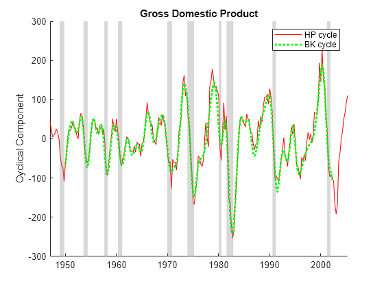
Baxter and King note that this close correspondence between the cyclical components does not hold true for all series because the Hodrick-Prescott filter allows unlimited high-frequency variation into the cyclical component. Some macroeconomic series, such as the inflation rate, have significant high-frequency variation.

Load the Schwert macroeconomic series data set Data_SchwertMacro.mat. Extract the monthly Consumer Price Index (CPI) and transform it to an inflation rate series.

load Data_SchwertMacro
CPI = DataTableMth.CPI;
INFRate = 100*diff(CPI)./CPI(1:end-1);
tINF = datetime(datesMth(2:end),ConvertFrom="datenum");

Apply the Hodrick-Prescott and Baxter-King filters to the US inflation rate series. Use the parameter settings recommended for monthly data. Visually compare the cyclical components.

[~,INFHPCycle] = hpfilter(INFRate,Smoothing=14400);
[~,INFBKCycle] = bkfilter(INFRate,LowerCutoff=18,UpperCutoff=96, ...
    LagLength=36);

figure
hold on
plot(tINF,INFHPCycle,"r")
plot(tINF,INFBKCycle,"g:",LineWidth=2)
recessionplot
hold off
ylabel("Cyclical Component")
title("Inflation Rate")
legend(["HP Cycle" "BK Cycle"])

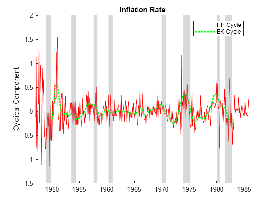
The absolute variation is significantly greater in the Hodrick-Prescott cycle.

Christiano-Fitzgerald Filter

Christiano and Fitzgerald [4] describe another bandpass filter to extract middle-frequency business cycles. The cffilter function implements the Christiano-Fitzgerald filter.

Differences between the Baxter-King and Christiano-Fitzgerald bandpass filters are mostly technical (each optimizes a different objective function), not functional (both filters specify lower and upper cutoff periods for the cycle). The Christiano-Fitzgerald filter produces asymptotically optimal finite-sample approximations to an ideal bandpass filter. A caveat is that it "is optimal under the (most likely, false) assumption that the data are generated by a pure random walk."

To evaluate the performance of the filter under the pure random walk assumption, generate a path from a random walk model, with a drift component to introduce a trend.

RW0 = 0;     % Initial value
drift = 0.2; % Drift component
sigma = 0.2; % Innovations standard deviation

rng(1); % For reproducibility
RW = RW0*ones(100,1);
for tRW = 2:100
    RW(tRW) = RW(tRW-1) + drift + sigma*randn; % Random walk with unit root
end

plot(RW)
title("Random Walk with Drift")

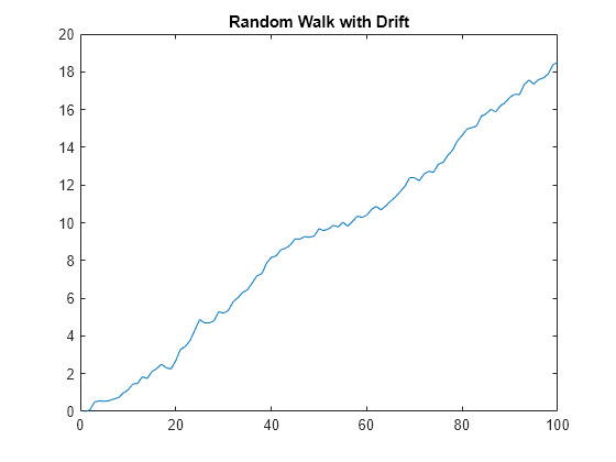
Compare the Baxter-King and Christiano-Fitzgerald bandpass filters under the random walk assumption, treating the data as quarterly. When a series is trending, cffilter must estimate an additional drift parameter. Therefore, specify that the series has drift by setting the Drift name-value argument to true. The Christiano-Fitzgerald filter avoids end-trimming of data by using an asymmetric, time-varying moving average (the default FilterType="asymmetric") to smooth the data and extract the trend component, so it does not require a LagLength name-value argument. The asymmetric filter can cause some phase shifting in the cycle.

[~,RWBKCycle] = bkfilter(RW);
[~,RWCFCycle] = cffilter(RW,Drift=true);

figure
hold on
plot(RWBKCycle,"g:",LineWidth=2)
plot(RWCFCycle,"c",LineWidth=2)
hold off
ylabel("Cyclical Component")
title("Random Walk with Drift")
legend(["BK cycle" "CF cycle"])

The presence of random walks in economic data, and more generally unit roots in autoregressive models, is a subject of continuing debate in econometrics. The assumption has significant consequences for long-term forecasting. Regarding filter performance, however, Christiano and Fitzgerald claim that their method "is nearly optimal for the type of time series representations that fit US data on interest rates, unemployment, inflation, and output" and consequently "though it is only optimal for one particular time series representation, nevertheless works well for standard macroeconomic time series."

Compare the two bandpass filters on the GDP output data. Because the raw GDP data exhibits a drift, specify estimating the drift component.

[~,GDPBKCycle] = bkfilter(GDP);
[~,GDPCFCycle] = cffilter(GDP,Drift=true);

figure
hold on
plot(tGDP,GDPBKCycle,"g:",LineWidth=2)
plot(tGDP,GDPCFCycle,"c",LineWidth=2)
recessionplot
hold off
ylabel("Cyclical Component")
title("Gross Domestic Product")
legend(["BK cycle" "CF cycle"])

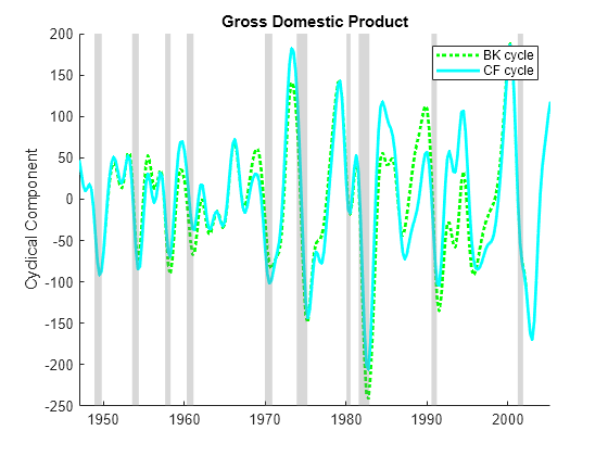
Differences between the Baxter-King and Christiano-Fitzgerald cycles appear at data endpoints, where the Baxter-King method clips the cycle by lag and lead lengths. For the GDP data, you can also see differences in the amplitudes of the cyclical swings, which determine turning points for periods of recession and expansion.

For a thorough analysis of economic data, you can use the two filters, with their different optimizations, to complement each other.

One-Sided Hodrick-Prescott Filter

The standard Hodrick-Prescott filter computes a two-sided, centered difference to estimate a second derivative at time t, using both past and future values of the input series. As such, the filter is often applied to historical data. However, this noncausality can lead to end effects that give the filtered data a retrospective, and artificial, predictive power.

Stock and Watson [15] suggest that the noncausality in the Hodrick-Prescott filter can distort forecast results. To address this distortion, they consider a one-sided version of the filter that uses only current and previous values of the input series. The one-sided filter does not revise outputs when new data becomes available. The one-sided filter aims to produce robust forecast performance rather than extract a secular trend. This revised goal reframes the notion of business cycle.

The hpfilter function, with name-value argument FilterType set to "one-sided", implements the one-sided Hodrick-Prescott filter.

Compare the two versions of the Hodrick-Prescott filter on the GDP output data.

[~,GDPHP2Cycle] = hpfilter(GDP);
[~,GDPHP1Cycle] = hpfilter(GDP,Smoothing=1600,FilterType="one-sided");

figure
hold on
plot(tGDP,GDPHP2Cycle,"r")
plot(tGDP,GDPHP1Cycle,"r:",LineWidth=2)
recessionplot
hold off
ylabel("Cyclical Component")
title("Gross Domestic Product")
legend(["Two-sided HP cycle" "One-sided HP cycle"])

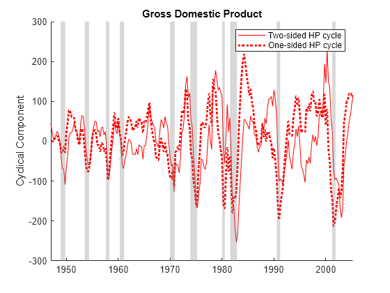
The two cycles lead to distinct calibrations of forecasting models (see Evaluate Filter Performance).

Hamilton Filter

Hamilton [9] expresses concern about use of the Hodrick-Prescott filter, including ad hoc methods for setting the smoothing parameter and the potential for producing spurious end effects. These concerns have been addressed in, for example, [1], [4], [13], and [15].

Hamilton presents what he calls a "better alternative," claiming it "offers a robust approach to detrending that achieves all the objectives sought by users of the HP filter with none of its drawbacks." His method is "a regression of the variable at date t + h on the four most recent values as of date t," with the business cycle defined by the forecast error: "How different is the value at $\mathit{t}+\mathit{h}$ from the value that we would have expected to see based on its behavior through date $\mathit{t}$?" The method is related to the time series decomposition in [2].

The hfilter function implements the Hamilton filter.

Compare the Hamilton filter with the similarly forecast-oriented one-sided Hodrick-Prescott filter. Apply the filters to the GDP output data. Use the default values of the following optional name-value arguments of hfilter:

• LeadLength —The horizon $\mathit{h}$ of the response variable in the regression. The default is 8.

• LagLength — The number of recent values to use as predictor variables in the regression. The default is 4.

[~,GDPHCycle] = hfilter(GDP);
[~,GDPHP1Cycle] = hpfilter(GDP,FilterType="one-sided");

figure
hold on
plot(tGDP,GDPHCycle,"k")
plot(tGDP,GDPHP1Cycle,"r:",LineWidth=2)
recessionplot
hold off
ylabel("Cyclical Component")
title("Gross Domestic Product")
legend(["H cycle" "HP1 cycle"])

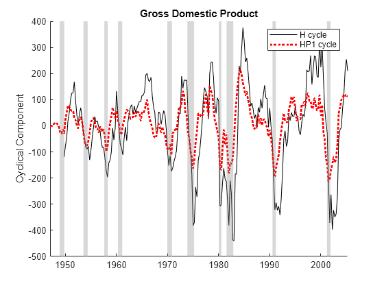
Because hfilter requires lags of the input variable, the function trims observations at the beginning of the data. The Hamilton cycle shows more distinct departures during historical recessions and expansions, which identify turning points and calibrate forecasting models.

Evaluate Filter Performance

Despite the different approaches, the filters in this example often identify similar cycles in economic data, reinforcing the idea of a true business cycle that exists in the data-generating process (DGP). The plots show estimated cycles under the different assumptions and optimizations characterizing the individual filters. However, the plots do not show how well each filter meets its own objectives or captures the DGP cycle.

To evaluate relative performance, you must measure outcomes on the same terms. For example, the Baxter-King and Christiano-Fitzgerald filters both approximate ideal bandpass filters for isolating a mid-range of frequencies. Accordingly, compare the performance of these two filters by seeing which frequencies appear in the extracted cycle. A periodogram, computed by the discrete Fourier Transforms, shows the power of different frequencies in the filtered series, conditional on filter parameter settings.

Compute the power spectrum of the cyclical components of the US GDP returned by the Baxter-King and Christiano-Fitzgerald filters (GDPBKCycle and GDPCFCycle). Specify comparable settings.

fs = 1; % Sample frequency (per quarter)

GDPBKCycle = rmmissing(GDPBKCycle);
nBK = length(GDPBKCycle);
DFTBK = fft(GDPBKCycle); 
fBK = (0:nBK-1)*(fs/nBK);     % Frequency range
PBK = DFTBK.*conj(DFTBK)/nBK; % Power

nCF = length(GDPCFCycle);
DFTCF = fft(GDPCFCycle); 
fCF = (0:nCF-1)*(fs/nCF);     % Frequency range
PCF = DFTCF.*conj(DFTCF)/nCF; % Power

Compare the periodograms of the two series.

figure
hold on
plot(fBK,log(PBK),"g:",LineWidth=2)
plot(fCF,log(PCF),"c",LineWidth=2)
hold off
xline(fs/6,"r")  % Burns and Mitchell upper frequency
xline(fs/32,"r") % Burns and Mitchell lower frequency
xlim([0 fs/2])
xlabel("Frequency")
ylabel("Log Power")
title("Periodogram")
legend(["BK cycle" "CF cycle" "Cutoffs"])

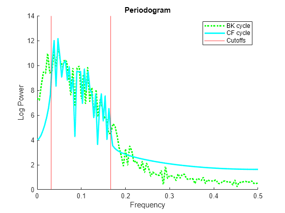
Both filters concentrate power in the specified frequency band. On the GDP data, the Christiano-Fitzgerald filter is slightly more successful at removing the low-frequency trend components, while the Baxter-King filter is more successful at removing high-frequency noise.

Similarly, compare the one-sided Hodrick-Prescott filter with the Hamilton filter based on their forecasting goals. Use the following procedure:

1. Fit a two-state (recession/expansion) Markov-switching model to the extracted cycles in the first two-thirds of the GDP data.

2. Forecast each series into the final one-third of the data.

Partition the data into estimation and forecast samples.

n = length(GDP);
nEst = floor((2/3)*n);
nFor = n-nEst;
GDPEst = GDP(1:nEst);     % Estimation sample
tGDPEst = tGDP(1:nEst);
GDPFor = GDP(nEst+1:end); % Forecast sample
tGDPFor = tGDP(nEst+1:end);

Filter the cycles from the estimation sample using the one-sided Hodrick-Prescott and Hamilton filters. Preprocess the cycles by trimming any leading and trailing NaN values and scaling the series to improve estimation.

[~,GDPEstHCycle] = hfilter(GDPEst);
GDPEstHCycle = rmmissing(GDPEstHCycle);
GDPEstHCycleS = GDPEstHCycle/100;

[~,GDPEstHP1Cycle] = hpfilter(GDPEst,FilterType="one-sided");
GDPEstHP1CycleS = GDPEstHP1Cycle/100;

Fit a two-state Markov-switching model with AR(1) submodels to each estimation sample cycle. For more details on Markov-switching models, see Creating Markov-Switching Dynamic Regression Models.

% Partially specified models for estimation
P = NaN(2);
mc = dtmc(P);
mdl = arima(1,0,0);
Mdl = msVAR(mc,[mdl; mdl]);

% Fully specified models of initial values
P0 = 0.5*ones(2);
mc0 = dtmc(P0);
mdl01 = arima('Constant',1,'AR',0.5,'Variance',1);
mdl02 = arima('Constant',-1,'AR',0.5,'Variance',1);
Mdl0 = msVAR(mc0,[mdl01; mdl02]);

% Fit models to scaled cycles.
EstMdlH = estimate(Mdl,Mdl0,GDPEstHCycleS);
EstMdlHP1 = estimate(Mdl,Mdl0,GDPEstHP1CycleS);

Extract cycles from the forecast sample using the one-sided Hodrick-Prescott and Hamilton filters. Preprocess the cycles by scaling the series to match the estimation sample scale.

[~,GDPForHCycle] = hfilter(GDPFor);
GDPForHCycleS = GDPForHCycle/100;

[~,GDPForHP1Cycle] = hpfilter(GDPFor,FilterType="one-sided");
GDPForHP1CycleS = GDPForHP1Cycle/100;

Provide optimal point forecasts of the switching models into the forecast period. Supply the scaled estimation cycles as presample data to initialize the forecasts.

fH = forecast(EstMdlH,GDPEstHCycleS,nFor);
fHP1 = forecast(EstMdlHP1,GDPEstHP1CycleS,nFor);

Compare the forecasts with the filtered cycles.

figure
hold on
h1 = plot(tGDPEst(end-length(GDPEstHCycle)+1:end),GDPEstHCycleS,"k");
h2 = plot(tGDPFor,GDPForHCycleS,"k--");
h3 = plot(tGDPEst,GDPEstHP1CycleS,"r:",LineWidth=2);
h4 = plot(tGDPFor,GDPForHP1CycleS,"r--");
h5 = plot(tGDPFor,fH,"k",LineWidth=2);
h6 = plot(tGDPFor,fHP1,"r",LineWidth=2);
yfill = [ylim fliplr(ylim)];
xfill = [tGDPEst([end end])' tGDPFor([end end])'];
patch(xfill,yfill,'k',FaceAlpha=0.05)
hold off
ylabel("Scaled Cyclical Component")
title("GDP Forecasts")
names = ["H estimation cycle" "H forecast cycle" ...
    "HP1 estimation cycle" "HP1 forecast cycle" ...
    "H forecast" "HP1 forecast"];
legend([h1 h2 h3 h4 h5 h6],names,Location="northwest")

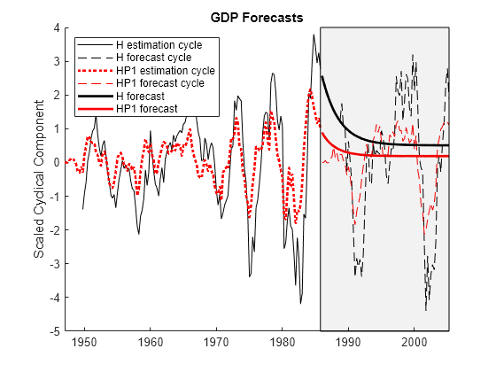
The forecasts, though different, are comparable over a business cycle horizon. However, the forecasts depend as much on the model fit to the cycles and the forecasting method employed as they do on the cycles extracted by the filters. As a result, a clear measure of filter performance is difficult to determine from this analysis (see also [14]).

The difficulty is essential. The extracted cycles cannot be compared to measurable data. The filters do not identify true cycles, but cycles built into their respective designs. Absolute filter performance becomes self-referential, evaluated on specific assumptions about the nature of the business cycle and the data-generating process.

Hodrick [10] addresses concerns about the Hodrick-Prescott filter by comparing it to other filters in the context of a variety of data-generating processes relevant to economic time series. He considers simple processes, such as random walks and ARIMA models, with no distinction between trend and cyclical components, and more complex processes, such as unobserved components models, where trend and cyclical components are modeled explicitly. When built into the model, cycles serve as proxies for true cycles in the macroeconomy, and simulations provide measurable data for comparison. Hodrick claims that "as the time series become more complex, the performance of the HP and BK filters more closely characterize the underlying cyclical frameworks than the H filter."

To illustrate Hodrick's investigation, simulate an unobserved components model of the GDP, as in [5], calibrated with parameter settings in [10].

numSim = 100;
rng(1); % For reproducibility

% Preallocate
coditionalMean = ones(numSim,1);
simCycle = ones(numSim,1);
simTrend = ones(numSim,1);

% Coefficients from Hodrick [10]
sigma1 = 0.021;
sigma2 = 0.603;
sigma3 = 0.545;
ARCycle = [1.510,-0.565];

% Unobserved components model
for t = 3:numSim
    coditionalMean(t) = coditionalMean(t-1) + sigma1*randn; % Random walk
    simCycle(t) = ARCycle*[simCycle(t-1);simCycle(t-2)] + sigma2*randn; % ARIMA(2,0,0)
    simTrend(t) = simTrend(t-1) + coditionalMean(t-1) + sigma3*randn;
end

simData = simCycle + simTrend; % DGP = Cycle + Trend

figure
plot(simData)
title("Simulated GDP Data")

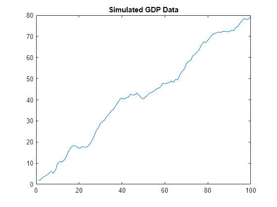
The simulated data is comparable to empirical GDP data.

Apply the two-sided Hodrick-Prescott, Baxter-King, and Hamilton filters to the simulated data.

[~,simHPCycle] = hpfilter(simData);
[~,simBKCycle] = bkfilter(simData);
[~,simHCycle] = hfilter(simData);

figure
hold on
h0 = plot(simCycle,LineWidth=2);
h1 = plot(simHPCycle,"r");
h2 = plot(simBKCycle,"g:",LineWidth=2);
h3 = plot(simHCycle,"k--");
hold off
names = ["DGP" "HP" "BK" "H"];
legend([h0 h1 h2 h3],names,Location="northwest")
title("Cycle Estimates")

The cycles identified by the Hodrick-Prescott and Baxter-King filters mostly follow one another, while the Hamilton cycle swings more widely. Because the DGP cycle, simCycle, is built into the model, it is available for comparison when evaluating filter performance.

Plot pairwise correlations of the cycles.

corrplot([simCycle simHPCycle simBKCycle simHCycle],VarNames=names)

In this simulation of the GDP, the HP and BK cycles are tightly correlated with each other, and they are more strongly correlated with the DGP than the Hamilton cycle. For an analysis with similar conclusions, see [12].

Hodrick summarizes by saying, "Consequently, the most desirable approach to decomposing a time series into growth and cyclical components and hence the advice that one would give to someone that wants to detrend a series to focus on cyclical fluctuations clearly depends on the underlying model that one has in mind. For GDP, if one thinks that growth is caused by slowly moving changes in demographics, like population growth and changes in rates of labor force participation, as well as slowly moving changes in the productivity of capital and labor, then the filtering methods of Hodrick and Prescott and Baxter and King seem like the superior way to model the cyclical component."

Summary

The Hodrick-Prescott filter focuses on the identification of a slowly moving, easily computable trend component in macroeconomic time series. The Baxter-King and Christiano-Fitzgerald filters focus on frequency domain specifications of the cycle. The one-sided Hodrick-Prescott and Hamilton filters are more concerned with forecast performance for real-time analysis. Each filter is based on a particular definition of the business cycle, and choosing among them depends on what you aim to capture in the cycle.

Because you cannot measure true business cycles, you must evaluate each filter relative to its own goals. Simulation studies show that different options perform better or worse depending on the nature of the data-generating process. Researchers often have a specific model in mind, based on economic theory, and they should choose a filter that is best adapted to that setting. Otherwise, practitioners should look to the filters presented in this example for a variety of robust, well-regarded options, suitable for comparative analyses.

References

[1] Baxter, Marianne, and Robert G. King. "Measuring Business Cycles: Approximate Band-Pass Filters for Economic Time Series." Review of Economics and Statistics 81, no. 4 (November 1999): 575–93. https://doi.org/10.1162/003465399558454.

[2] Beveridge, Stephen, and Charles R. Nelson. "A New Approach to Decomposition of Economic Time Series into Permanent and Transitory Components with Particular Attention to Measurement of the 'Business Cycle.'" Journal of Monetary Economics 7 (January 1981): 151–74. https://doi.org/10.1016/0304-3932(81)90040-4.

[3] Burns, Arthur F., and Wesley C. Mitchell. Measuring Business Cycles. Cambridge, MA: National Bureau of Economic Research, 1946.

[4] Christiano, Lawrence J., and Terry J. Fitzgerald. "The Band Pass Filter." International Economic Review 44 (May 2003): 435–65. https://doi.org/10.1111/1468-2354.t01-1-00076.

[5] Clark, Peter K. "The Cyclical Component of U. S. Economic Activity." The Quarterly Journal of Economics 102, no. 4 (November 1987): 797–814. https://doi.org/10.2307/1884282.

[6] Cogley, Timothy, and James M. Nason. "Effects of the Hodrick-Prescott Filter on Trend and Difference Stationary Time Series Implications for Business Cycle Research." Journal of Economic Dynamics and Control 19, no. 1 (January1995): 253–78. https://doi.org/10.1016/0165-1889(93)00781-X.

[7] de Jong, Robert M., and Neslihan Sakarya. "The Econometrics of the Hodrick-Prescott Filter." Review of Economics and Statistics 98, no. 2 (May 2016): 310–17. https://doi.org/10.1162/REST_a_00523.

[8] Granger, Clive W. J. "The Typical Spectral Shape of an Economic Variable." Econometrica 34, no. 1 (January 1966): 150–61. https://doi.org/10.2307/1909859.

[9] Hamilton, James D. "Why You Should Never Use the Hodrick-Prescott Filter." The Review of Economics and Statistics 100 (December 2018): 831–43. https://doi.org/10.1162/rest_a_00706.

[10] Hodrick, Robert J. "An Exploration of Trend-Cycle Decomposition Methodologies in Simulated Data." National Bureau of Economic Research Working Paper No. w26750. Social Science Research Network (February 2020). https://papers.ssrn.com/abstract=3539317.

[11] Hodrick, Robert J., and Edward C. Prescott. "Postwar U.S. Business Cycles: An Empirical Investigation." Journal of Money, Credit and Banking 29, no. 1 (February 1997): 1–16. https://doi.org/10.2307/2953682.

[12] Morley, James C., Charles R. Nelson, and Eric Zivot. "Why Are the Beveridge-Nelson and Unobserved-Components Decompositions of GDP So Different?" Review of Economics and Statistics 85, no. 2 (May 2003): 235–43. https://doi.org/10.1162/003465303765299765.

[13] Ravn, Morton O., and Harald Uhlig. "On Adjusting the Hodrick-Prescott Filter for the Frequency of Observations." The Review of Economics and Statistics 84 , no. 2 (May 2002): 371–76. https://doi.org/10.1162/003465302317411604.

[14] Shackleton, Robert. "Estimating and Projecting Potential Output Using CBO's Forecasting Growth Model." Congressional Budget Office Working Paper No. 2018-03 (February 2018). https://www.cbo.gov/publication/53558.

[15] Stock, James H., and Mark W. Watson. "Forecasting Inflation." Journal of Monetary Economics 44, no. 2 (October 1999): 293–335. https://doi.org/10.1016/S0304-3932(99)00027-6.