kpsstest
KPSS test for stationarity
Syntax
Description
h = kpsstest(y)
StatTbl = kpsstest(Tbl)Tbl. To select a different variable in
Tbl to test, use the
DataVariable name-value
argument.
[___] = kpsstest(___,
specifies options using one or more name-value arguments in
addition to any of the input argument combinations in previous syntaxes.
Name=Value)kpsstest returns the output argument combination for the
corresponding input arguments.
Some options control the number of tests to conduct. The following
conditions apply when kpsstest conducts
multiple tests:
For example,
kpsstest(Tbl,DataVariable="GDP",Alpha=0.025,Lags=[0
                                        1])
conducts two tests, at a level of significance
of 0.025, for the presence of a unit root in the variable
GDP of the table Tbl.
The first test includes 0 autocovariance lags in
the Newey-West estimator of the long-run variance and the second
test includes 1 autocovariance lag.
Examples
Test a time series for a unit root using the default options of kpsstest. Input the time series data as a numeric vector.
Load the Nelson-Plosser macroeconomic series data set. Plot the real gross national product (RGNP).
load Data_NelsonPlosser
rgnp = DataTable.GNPR;
dt = datetime(dates,ConvertFrom="datenum");

plot(dt,rgnp)
title("Real Gross National Product")
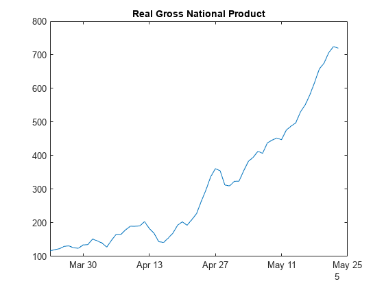
The series exhibits exponential growth.
Linearize the RGNP series.
linRGNP = log(rgnp);
Assess the null hypothesis of the KPSS test, which is that the series is trend stationary. Use default options.
h = kpsstest(linRGNP)
h = logical
   1
h = 1 indicates that, at a 5% level of significance, the test rejects the null hypothesis that the linearized Real GNP series is trend stationary, which suggests that the series is unit root nonstationary.
Load the Nelson-Plosser Macroeconomic series data set, and linearize the RGNP series.
load Data_NelsonPlosser
linRGNP = log(DataTable.GNPR);
Assess the null hypothesis that the series is trend stationary. Return the test decision, -value, test statistic, and critical value.
[h,pValue,stats,cValue] = kpsstest(linRGNP)
h = logical
   1
pValue =
0.0100
stats =
0.6299
cValue =
0.1460
Test whether a time series, which is one variable in a table, is trend stationary using the default options.
Load the Nelson-Plosser macroeconomic series data set, which contains annual measurements of macroeconomic variables in the table DataTable. Linearize the RGNP series by applying the log transformation, and store the result in DataTable.
load Data_NelsonPlosser
DataTable.LinRGNP = log(DataTable.GNPR);
DataTable.Properties.VariableNames{end}
ans = 'LinRGNP'
Test the null hypothesis that the linearized RGNP series is trend stationary.
StatTbl = kpsstest(DataTable)
StatTbl=1×7 table
                h      pValue     stat      cValue    Lags    Alpha    Trend
              _____    ______    _______    ______    ____    _____    _____

    Test 1    true      0.01     0.62989    0.146      0      0.05     true
kpsstest returns test results and settings in the table StatTbl, where variables correspond to test results (h, pValue, stat, and cValue) and settings (Lags, Alpha, Trend), and rows correspond to individual tests (in this case, kpsstest conducts one test).
By default, kpsstest tests the last variable in the table. To select a variable from an input table to test, set the DataVariable option.
Conduct multiple tests on the linearized RGNP series that reproduce the first row of the second half of Table 5 in [2].
Load the Nelson-Plosser macroeconomic series data set, which contains annual measurements of macroeconomic variables in the table DataTable. Apply the log transformation to all variables in the table.
load Data_NelsonPlosser
LogDT = varfun(@log,DataTable);
LogDT.Properties.VariableNames{end}
ans = 'log_SP'
varfun applies log to all variables in DataTable, prepends log_ to all transformed variable names, and stores the result in the table LogDT. The final variable is the log of the stock price index series (SP).
Assess the null hypothesis that the linearized RGNP series is trend stationary over a range of lags. Specify the variable name of the linearized RGNP series log_GNPR.
lags = (0:8);
StatTbl = kpsstest(LogDT,DataVariable="log_GNPR",Lags=lags)StatTbl=9×7 table
h pValue stat cValue Lags Alpha Trend
_____ ________ _______ ______ ____ _____ _____
Test 1 true 0.01 0.62989 0.146 0 0.05 true
Test 2 true 0.01 0.33666 0.146 1 0.05 true
Test 3 true 0.01 0.24209 0.146 2 0.05 true
Test 4 true 0.0169 0.1976 0.146 3 0.05 true
Test 5 true 0.027579 0.17291 0.146 4 0.05 true
Test 6 true 0.04015 0.15782 0.146 5 0.05 true
Test 7 true 0.048417 0.1479 0.146 6 0.05 true
Test 8 false 0.05886 0.14122 0.146 7 0.05 true
Test 9 false 0.066757 0.13695 0.146 8 0.05 true
The tests corresponding to 0 lags 2 produce -values that are less than 0.01. For 2 < lags < 7, the tests indicate sufficient evidence to suggest that log RGNP is unit root nonstationary (as opposed to the series being trend stationary) at the default 5% level.
Test whether the wage series in the manufacturing sector (1900–1970) has a unit root. Use the advice in [2] to select the number of lags in the Newey-West estimator of the coefficient standard errors.
Load the Nelson-Plosser macroeconomic data set. Remove all missing values from the data relative to the wage series WN.
load Data_NelsonPlosser
[DataTable,idx] = rmmissing(DataTable,DataVariables="WN");
dt = dates(~idx);
Compute the effective sample size and its square root, where the latter is approximately the number of lags recommended for the Newey-West estimator.
T = height(DataTable);
sqrtT = sqrt(T);
Plot the wage series.
plot(dt,DataTable.WN)
title("Wages")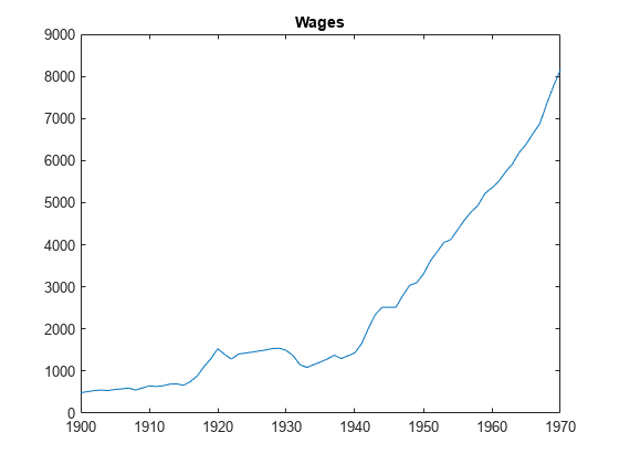
The wage series appears to grow exponentially.
Linearize the wages series by applying the log transformation to all variables in the table.
LogDT = varfun(@log,DataTable);
plot(dt,LogDT.log_WN)
title("Log Wages")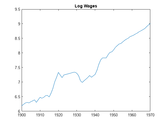
The log wage series appears to have a linear trend.
Test the null hypothesis that the log wage series is trend stationary (no unit root) against the alternative hypothesis that the log wage series is difference stationary. Conduct the test by setting a range of lags for the Newey-West estimator around .
StatTbl = kpsstest(LogDT,DataVariable="log_WN",Lags=7:10)StatTbl=4×7 table
h pValue stat cValue Lags Alpha Trend
_____ ______ ________ ______ ____ _____ _____
Test 1 false 0.1 0.10678 0.146 7 0.05 true
Test 2 false 0.1 0.10074 0.146 8 0.05 true
Test 3 false 0.1 0.096634 0.146 9 0.05 true
Test 4 false 0.1 0.094058 0.146 10 0.05 true
All tests fail to reject the null hypothesis that the log wages series is trend stationary.
The -values are larger than 0.1. The software compares the test statistic to critical values and computes -values that it interpolates from tables in [2].
Load the Nelson-Plosser macroeconomic series data set. Apply the log transformation to all variables in the table.
load Data_NelsonPlosser
LogDT = varfun(@log,DataTable);
Assess the null hypothesis that the linearized RGNP series is trend stationary. Use the Trend option to conduct the test with (true) and without (false) a deterministic time trend term in the response model. Return the regression statistics.
[~,reg] = kpsstest(LogDT,DataVariable="log_GNPR",Trend=[true false]);reg is a structure array of length 2 with fields that store the OLS regression results. Each element corresponds to a test.
Compare the coefficient estimates.
withTrend = reg(1).coeff
withTrend = 2×1

    4.5834
    0.0310
woTrend = reg(2).coeff
woTrend =
5.5595
For the first test, the response model for the regression includes a trend term, so the regression coefficients withTrend include a model intercept (under the null hypothesis) 4.5834 and the coefficient of the time trend 0.0310. For the second test, the response model includes an intercept only for the regression, so the intercept woTrend is 5.5595.
Display the coefficient standard errors for the first test.
reg(1).se
ans = 2×1

    0.0344
    0.0010
The Lags option includes autocovariance lags in the Newey-West estimator of the long-run variance. Therefore, the option does not affect the estimated OLS coefficients, standard errors, or MSE.
Conduct a KPSS test for each lag from 0 through 4. Compare the standard OLS and the Newey-West estimates.
lags = 0:4;
[~,regLags] = kpsstest(LogDT,DataVariable="log_GNPR",Lags=lags);

coeffs = table(regLags.coeff,VariableNames="Lags_"+lags, ...
    RowNames=["Intercept" "Trend"]);
se = table(regLags.se,VariableNames="Lags_"+lags, ...
    RowNames=["SE_Intercept" "SE_Trend"]);
mse = table(regLags.MSE,VariableNames="Lags_"+lags, ...
    RowNames="MSE");
nw = table(regLags.NWEst,VariableNames="Lags_"+lags, ...
    RowNames="NWVar");
[coeffs; se; mse; nw]
ans=6×5 table
                      Lags_0        Lags_1        Lags_2        Lags_3        Lags_4
                    __________    __________    __________    __________    __________

    Intercept           4.5834        4.5834        4.5834        4.5834        4.5834
    Trend             0.030988      0.030988      0.030988      0.030988      0.030988
    SE_Intercept       0.03443       0.03443       0.03443       0.03443       0.03443
    SE_Trend        0.00095035    0.00095035    0.00095035    0.00095035    0.00095035
    MSE               0.017933      0.017933      0.017933      0.017933      0.017933
    NWVar             0.017354       0.03247      0.045154      0.055321      0.063222
Input Arguments
Name-Value Arguments
Output Arguments
More About
Tips
To draw valid inferences from a KPSS test, you must determine a suitable value for the
Lagsargument. The following methods can determine a suitable number of lags:Begin with a small number of lags, and then evaluate the sensitivity of the results by adding more lags.
Kwiatkowski et al. [2] suggest that a number of lags on the order of , where T is the effective sample size, is often satisfactory under both the null and the alternative.
For consistency of the Newey-West estimator, the number of lags must approach infinity as the sample size increases.
With a specific testing strategy in mind, determine the value of the
Trendargument by the growth characteristics of the input time series.If the input series grows, include a trend term by setting
Trendtotrue(default). This setting provides a reasonable comparison of a trend stationary null and a unit root process with drift.If a series does not exhibit long-term growth characteristics, exclude a trend term by setting
Trendtofalse.
Algorithms
Test statistics follow nonstandard distributions under the null, even asymptotically. Kwiatkowski et al. [2] use Monte Carlo simulations, for models with and without a trend, to tabulate asymptotic critical values for a standard set of significance levels between 0.01 and 0.1.
kpsstestinterpolates critical values and p-values from these tables.
References
[1] Hamilton, James D. Time Series Analysis. Princeton, NJ: Princeton University Press, 1994.
[2] Kwiatkowski, D., P. C. B. Phillips, P. Schmidt, and Y. Shin. “Testing the Null Hypothesis of Stationarity against the Alternative of a Unit Root.” Journal of Econometrics. Vol. 54, 1992, pp. 159–178.
Version History
Introduced in R2009b