Estimate ARIMAX Model Using Econometric Modeler App
This example shows how to specify and estimate an ARIMAX model
using the Econometric Modeler app. The data set, which is stored in
Data_CreditDefaults.mat, contains annual investment-grade
corporate bond default rates, among other predictors, from 1984 through 2004.
Consider modeling corporate bond default rates as a linear, dynamic function of the
other time series in the data set.
Import Data into Econometric Modeler
At the command line, load the Data_CreditDefaults.mat data
set.
load Data_CreditDefaultsFor more details on the data set, enter Description at the
command line.
At the command line, open the Econometric Modeler app.
econometricModeler
Alternatively, open the app from the apps gallery (see Econometric Modeler).
Import DataTimeTable into the app:
On the Modeler tab, in the Import section, click the Import button
 .
.In the Import Data dialog box, select the check box for the
DataTimeTablevariable.Click Import.
The variables, including IGD, appear in the
Time Series pane, and a time series plot containing all
the series appears in the Plot(AGE) figure window.
Assess Stationarity of Dependent Variable
In the Time Series pane, double-click
IGD. The value of IGD
appears in the Preview pane, and a time series plot for
IGD appears in the Plot(IGD)
figure window.
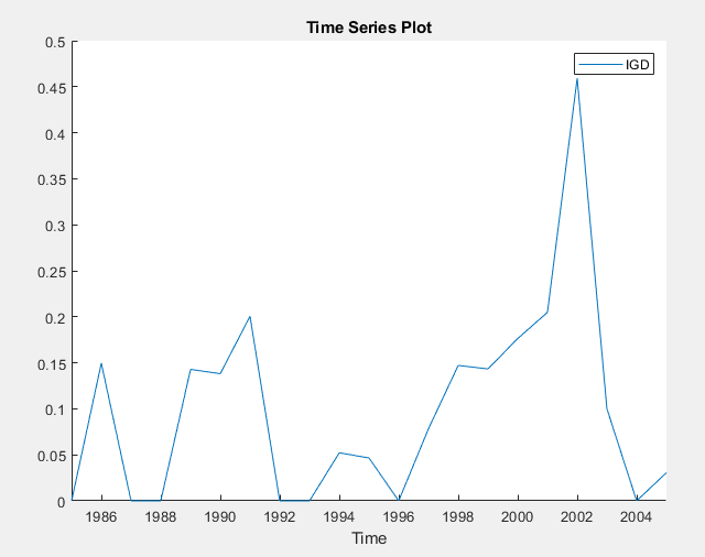
IGD appears to be stationary.
Assess whether IGD has a unit root by conducting a
Phillips-Perron test:
On the Modeler tab, in the Tests section, click Add Test > Phillips-Perron Test.
On the PP tab, in the Settings section, set Number of Lags to
1.In the Tests section, click Run Test.
The test results in the Results table of the PP(IGD) document.
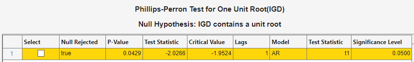
The test rejects the null hypothesis that IGD
contains a unit root.
Inspect Correlation and Collinearity Among Variables
Plot the pairwise correlations between variables.
Select all variables in the Time Series pane by clicking
AGE, then press Shift and clickSPR.Click the Plots tab, then click Corr.
A correlations plot appears in the Corr(AGE) figure window.
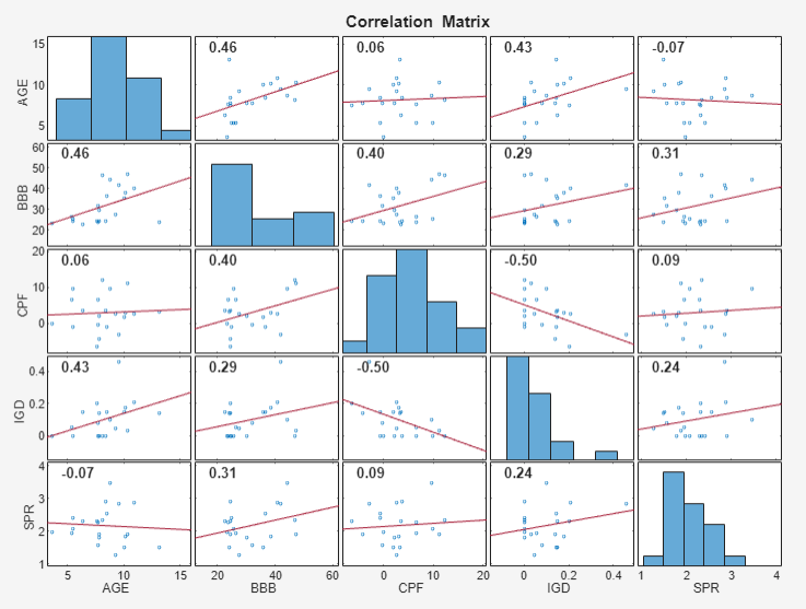
All predictors appear weakly associated with IGD.
You can test whether the correlation coefficients are significant by using
corrplot at the command line.
Assess whether any variables are collinear by performing Belsley collinearity diagnostics:
In the Time Series pane, select all variables.
Click the Modeler tab. Then, in the Tests section, click Add Test > Belsley Collinearity Diagnostics.
Tabular results appear in the Collin(AGE) document.
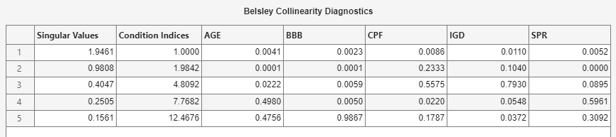
None of the condition indices are greater than the condition-index tolerance
(30). Therefore, the variables do not exhibit
multicollinearity.
Specify and Estimate ARIMAX Model
Consider an ARIMAX(0,0,1) model for IGD containing
all predictors. Specify and estimate the model.
In the Time Series pane, click
IGD.Click the Modeler tab. Then, in the Models section, click the arrow to display the models gallery.
In the models gallery, in the ARIMA Models section, click ARIMAX.
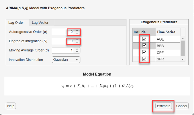
In the ARIMAX Model Parameters dialog box, on the Lag Order tab:
Set Autoregressive Order (p) to
0.Set Degree of Integration (D) to
0.
In the Predictors section, select the Include check box for each time series. Click Estimate.
The model variable
ARIMAX_IGDappears in the Models pane, its value appears in the Preview pane, and its estimation summary appears in the Fit(ARIMAX_IGD) document.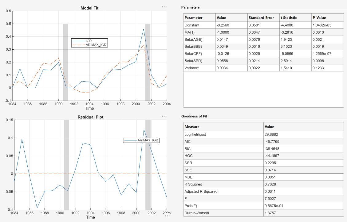
At a 0.10 significance level, all predictors and the MA coefficient are significant.
Close all figure windows and documents.
Check Goodness of Fit
Check that the residuals are normally distributed and uncorrelated by plotting a histogram, quantile-quantile plot, and ACF of the residuals.
In the Models pane, select
ARIMAX_IGD.On the Modeler tab, in the Diagnostics section, click Model Fit Diagnostics > Residual Histogram.
Click Model Fit Diagnostics > Residual Q-Q Plot.
Click Model Fit Diagnostics > Autocorrelation Function.
In the right pane, drag the Hist(ARIMAX_IGD) and QQ(ARIMAX_IGD) figure windows so that they occupy the upper two quadrants, and drag the ACF so that it occupies the lower two quadrants.
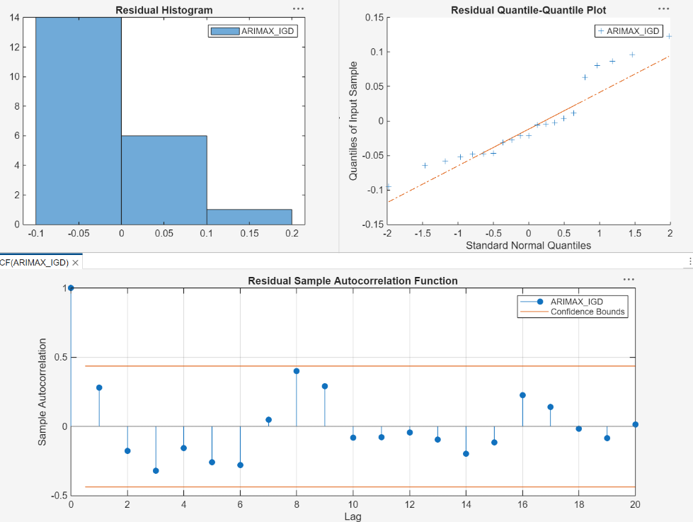
The residual histogram and quantile-quantile plots suggest that the residuals might not be normally distributed. According to the ACF plot, the residuals do not exhibit serial correlation. Standard inferences rely on the normality of the residuals. To remedy nonnormality, you can try transforming the response, then estimating the model using the transformed response.