conjugateblm
Bayesian linear regression model with conjugate prior for data likelihood
Description
The Bayesian linear regression
model object conjugateblm specifies that the joint prior
distribution of the regression coefficients and the disturbance variance, that is,
(β, σ2) is the
dependent, normal-inverse-gamma conjugate model. The
conditional prior distribution of
β|σ2 is
multivariate Gaussian with mean μ and variance
σ2V. The prior
distribution of σ2 is inverse gamma with
shape A and scale B.
The data likelihood is where ϕ(yt;xtβ,σ2) is the Gaussian probability density evaluated at yt with mean xtβ and variance σ2. The specified priors are conjugate for the likelihood, and the resulting marginal and conditional posterior distributions are analytically tractable. For details on the posterior distribution, see Analytically Tractable Posteriors.
In general, when you create a Bayesian linear regression model object, it specifies the joint prior distribution and characteristics of the linear regression model only. That is, the model object is a template intended for further use. Specifically, to incorporate data into the model for posterior distribution analysis, pass the model object and data to the appropriate object function.
Creation
Description
PriorMdl = conjugateblm(NumPredictors)PriorMdl) composed of
NumPredictors predictors and an intercept, and sets
the NumPredictors property. The joint prior
distribution of (β,
σ2) is the dependent
normal-inverse-gamma conjugate model. PriorMdl is a
template that defines the prior distributions and the dimensionality of
β.
PriorMdl = conjugateblm(NumPredictors,Name,Value)NumPredictors) using name-value pair arguments.
Enclose each property name in quotes. For example,
conjugateblm(2,'VarNames',["UnemploymentRate";
                            "CPI"])
specifies the names of the two predictor variables in
the model.
Properties
Object Functions
estimate | Estimate posterior distribution of Bayesian linear regression model parameters |
simulate | Simulate regression coefficients and disturbance variance of Bayesian linear regression model |
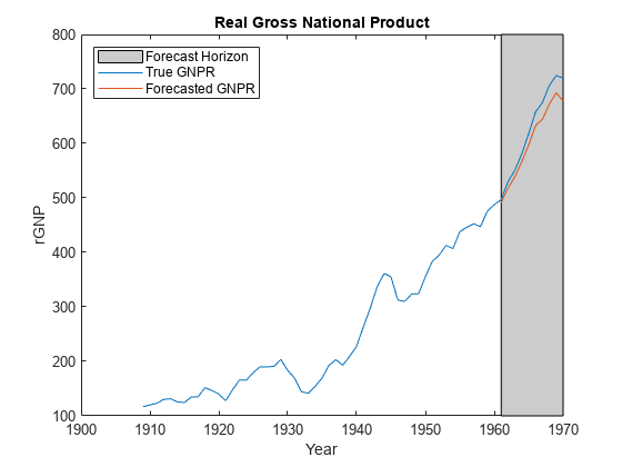
forecast | Forecast responses of Bayesian linear regression model |
plot | Visualize prior and posterior densities of Bayesian linear regression model parameters |
summarize | Distribution summary statistics of standard Bayesian linear regression model |
Examples
More About
Algorithms
You can reset all model properties using dot notation, for example, PriorMdl.V
= diag(Inf(3,1)). For property resets, conjugateblm does
minimal error checking of values. Minimizing error checking has the
advantage of reducing overhead costs for Markov chain Monte Carlo
simulations, which results in efficient execution of the algorithm.
Alternatives
The bayeslm function can create any supported prior model object for Bayesian linear regression.
Version History
Introduced in R2017a
