Choose ARMA Lags Using BIC

This example shows how to use the Bayesian information criterion (BIC) to select the degrees p and q of an ARMA model. Estimate several models with different p and q values. For each estimated model, output the loglikelihood objective function value. Input the loglikelihood value to aicbic to calculate the BIC measure of fit (which penalizes for complexity).

Simulate ARMA time series

Simulate an ARMA(2,1) time series with 100 observations.

Mdl0 = arima('Constant',0.2,'AR',{0.75,-0.4},...
               'MA',0.7,'Variance',0.1);
rng(5)
Y = simulate(Mdl0,100);

figure
plot(Y)
xlim([0,100])
title('Simulated ARMA(2,1) Series')

Plot Sample ACF and PACF

Plot the sample autocorrelation function (ACF) and partial autocorrelation function (PACF) for the simulated data.

figure
subplot(2,1,1)
autocorr(Y)
subplot(2,1,2)
parcorr(Y)

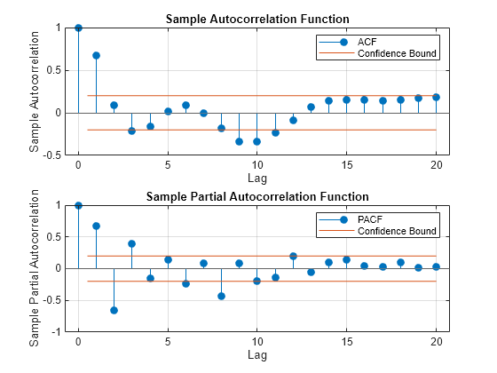
Both the sample ACF and PACF decay relatively slowly. This is consistent with an ARMA model. The ARMA lags cannot be selected solely by looking at the ACF and PACF, but it seems no more than four AR or MA terms are needed.

Fit ARMA(p,q) Models to Data

To identify the best lags, fit several models with different lag choices. Here, fit all combinations of p = 1,...,4 and q = 1,...,4 (a total of 16 models). Store the loglikelihood objective function and number of coefficients for each fitted model.

LogL = zeros(4,4); % Initialize
PQ = zeros(4,4);
for p = 1:4
    for q = 1:4
        Mdl = arima(p,0,q);
        [EstMdl,~,LogL(p,q)] = estimate(Mdl,Y,'Display','off');
        PQ(p,q) = p + q;
     end
end

Calculate BIC

Calculate the BIC for each fitted model. The number of parameters in a model is p + q + 1 (for the AR and MA coefficients, and constant term). The number of observations in the data set is 100.

logL = LogL(:);
pq = PQ(:);
[~,bic] = aicbic(logL,pq+1,100);
BIC = reshape(bic,4,4)

BIC = 4×4

  102.4215   96.2339  100.8005  100.3440
   89.1130   93.4895   97.1530   94.0615
   93.6770   93.2838  100.2190  103.4779
   98.2820  102.0442  100.3024  107.5245

In the output BIC matrix, the rows correspond to the AR degree (p) and the columns correspond to the MA degree (q). The smallest value is best.

minBIC = min(BIC,[],'all')

minBIC = 89.1130

[minP,minQ] = find(minBIC == BIC)

minP = 2

minQ = 1

The smallest BIC value is 89.1130 in the (2,1) position. This corresponds to an ARMA(2,1) model, which matches the model that generated the data.