誤差曲面を示すパターンの関連付け

ターゲット出力を使用して特定の入力に応答するように線形ニューロンの設計を行います。

X は、2 つの 1 要素入力パターン (列ベクトル) を定義します。T は、関連する 1 要素ターゲット (列ベクトル) を定義します。

X = [1.0 -1.2];
T = [0.5 1.0];

ERRSURF は、可能な重みとバイアスの値の y 範囲を使用して y ニューロンの誤差を計算します。PLOTES は、この誤差曲面と、その下の y 等高線図を併せてプロットします。最適な重みとバイアスの値は、誤差曲面の最低点が得られる値です。

w_range = -1:0.1:1;
b_range = -1:0.1:1;
ES = errsurf(X,T,w_range,b_range,'purelin');
plotes(w_range,b_range,ES);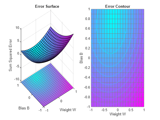

関数 NEWLIND は、最小誤差で実行される y ネットワークを設計します。

net = newlind(X,T);

SIM を使用して入力 X でネットワークをシミュレートします。その後、ニューロンの誤差を計算できます。SUMSQR は二乗誤差を合計します。

A = net(X)

A = 1×2

    0.5000    1.0000

E = T - A

E = 1×2

     0     0

SSE = sumsqr(E)

SSE = 
0

PLOTES は誤差曲面を再プロットします。PLOTEP は、SOLVELIN から返された重みとバイアスの値を使用してネットワークの "位置" をプロットします。プロットからわかるように、SOLVELIN は誤差が最小の解を見つけました。

plotes(w_range,b_range,ES);
plotep(net.IW{1,1},net.b{1},SSE);

これで、元の入力の 1 つである -1.2 でアソシエーターをテストし、ターゲットである 1.0 を返すかどうかを確認できます。

x = -1.2;
y = net(x)

y = 
1