Genetic Algorithm Search for Features in Mass Spectrometry Data

Open Script

This example shows how to use the Global Optimization Toolbox with the Bioinformatics Toolbox™ to optimize the search for features to classify mass spectrometry (SELDI) data.

Introduction

Genetic algorithms optimize search results for problems with large data sets. You can use the MATLAB® genetic algorithm function to solve these problems in Bioinformatics. Genetic algorithms have been applied to phylogenetic tree building, gene expression and mass spectrometry data analysis, and many other areas of Bioinformatics that have large and computationally expensive problems. This example searches for optimal features (peaks) in mass spectrometry data. We will look for specific peaks in the data that distinguish cancer patients from control patients.

Global Optimization Toolbox

First familiarize yourself with the Global Optimization Toolbox. The documentation describes how a genetic algorithm works and how to use it in MATLAB. To access the documentation, use the doc command.

doc ga

Preprocess Mass Spectrometry Data

The original data in this example is from the FDA-NCI Clinical Proteomics Program Databank. It is a collection of samples from 121 ovarian cancer patients and 95 control patients. For a detailed description of this data set, see [1] and [2].

This example assumes that you already have the preprocessed data OvarianCancerQAQCdataset.mat. However, if you do not have the data file, you can recreate by following the steps in the example Batch Processing of Spectra Using Sequential and Parallel Computing.

Alternatively, you can run the provided script msseqprocessing.m.

Load Mass Spectrometry Data into MATLAB®

Once you have the preprocessed data, you can load it into MATLAB.

load OvarianCancerQAQCdataset
whos

  Name          Size                Bytes  Class     Attributes

  MZ        15000x1                120000  double              
  Y         15000x216            25920000  double              
  grp         216x1                 25056  cell

There are three variables: MZ, Y, grp. MZ is the mass/charge vector, Y is the intensity values for all 216 patients (control and cancer), and grp holds the index information as to which of these samples represent cancer patients and which ones represent normal patients. To visualize this data, see the example Identifying Significant Features and Classifying Protein Profiles.

Initialize the variables used in the example.

[numPoints, numSamples] = size(Y); % total number of samples and data points
id = grp2idx(grp);  % ground truth: Cancer=1, Control=2

Create a Fitness Function for the Genetic Algorithm

A genetic algorithm requires an objective function, also known as the fitness function, which describes the phenomenon that we want to optimize. In this example, the genetic algorithm machinery tests small subsets of M/Z values using the fitness function and then determines which M/Z values get passed on to or removed from each subsequent generation. The fitness function biogafit is passed to the genetic algorithm solver using a function handle. For the implementation details, see the provided script biogafit.m. In this example, biogafit maximizes the separability of two classes by using a linear combination of 1) the a-posteriori probability and 2) the empirical error rate of a linear classifier (classify). You can create your own fitness function to try different classifiers or alternative methods for assessing the performance of the classifiers.

Create an Initial Population

Users can change how the optimization is performed by the genetic algorithm by creating custom functions for crossover, fitness scaling, mutation, selection, and population creation. In this example you will use the biogacreate function written for this example to create initial random data points from the mass spectrometry data. For the implementation details, see the provided script biogacreate.m. The function header requires specific input parameters as specified by the GA documentation. There is a default creation function in the toolbox for creating initial populations of data points.

Set Genetic Algorithm Options

The GA function uses an options structure to hold the algorithm parameters that it uses when performing a minimization with a genetic algorithm. The optimoptions function will create this options structure. For the purposes of this example, the genetic algorithm will run only for 50 generations. However, you may set 'Generations' to a larger value.

options = optimoptions('ga','CreationFcn',{@biogacreate,Y,id},...
                       'PopulationSize',120,...
                       'Generations',50,...
                       'Display','iter')

options = 

  ga options:

   Set properties:
                     CreationFcn: {1×3 cell}
                         Display: 'iter'
                  MaxGenerations: 50
                  PopulationSize: 120

   Default properties:
             ConstraintTolerance: 1.0000e-03
                    CrossoverFcn: []
               CrossoverFraction: 0.8000
                      EliteCount: '0.05*PopulationSize'
                    FitnessLimit: -Inf
               FitnessScalingFcn: @fitscalingrank
               FunctionTolerance: 1.0000e-06
                       HybridFcn: []
         InitialPopulationMatrix: []
          InitialPopulationRange: []
             InitialScoresMatrix: []
             MaxStallGenerations: 50
                    MaxStallTime: Inf
                         MaxTime: Inf
                     MutationFcn: []
    NonlinearConstraintAlgorithm: 'auglag'
                       OutputFcn: []
                         PlotFcn: []
                  PopulationType: 'doubleVector'
                    SelectionFcn: []
                     UseParallel: 0
                   UseVectorized: 0

Run GA to Find 20 Discriminative Features

Use ga to start the genetic algorithm function. 100 groups of 20 datapoints each will evolve over 50 generations. Selection, crossover, and mutation events generate a new population in every generation.

% initialize the random generators to the same state used to generate the
% published example
rng('default')
nVars = 12;                          % set the number of desired features
FitnessFcn = {@biogafit,Y,id};       % set the fitness function
feat = ga(FitnessFcn,nVars,options); % call the Genetic Algorithm

feat = round(feat);
Significant_Masses = MZ(feat)

cp = classperf(classify(Y(feat,:)',Y(feat,:)',id),id);
cp.CorrectRate

Single objective optimization:
12 Variables

Options:
CreationFcn:       @biogacreate
CrossoverFcn:      @crossoverscattered
SelectionFcn:      @selectionstochunif
MutationFcn:       @mutationgaussian

                                  Best           Mean      Stall
Generation      Func-count        f(x)           f(x)    Generations
    1              240           2.827           8.928        0
    2              354           2.827           8.718        1
    3              468          0.9663           8.001        0
    4              582          0.9516           7.249        0
    5              696          0.9516           6.903        1
    6              810          0.4926           6.804        0
    7              924          0.4926           6.301        1
    8             1038         0.02443           5.215        0
    9             1152         0.02443            4.77        1
   10             1266         0.02101           4.084        0
   11             1380         0.02101           3.792        1
   12             1494         0.01854           3.437        0
   13             1608         0.01606            3.44        0
   14             1722         0.01372           2.768        0
   15             1836         0.01218            2.74        0
   16             1950         0.01204           2.471        0
   17             2064         0.01204           2.649        1
   18             2178         0.01189           2.326        0
   19             2292         0.01189           2.003        0
   20             2406          0.0118           2.341        0
   21             2520         0.01099           1.714        0
   22             2634         0.01094           1.828        0
   23             2748         0.01094            1.94        1
   24             2862         0.01094           2.285        2
   25             2976        0.009843           2.026        0
   26             3090        0.009843           1.899        1
   27             3204        0.009183           1.802        0
   28             3318        0.007877             1.5        0
   29             3432        0.007788           1.793        0
   30             3546        0.007788           1.756        1

                                  Best           Mean      Stall
Generation      Func-count        f(x)           f(x)    Generations
   31             3660        0.007091           1.719        0
   32             3774        0.006982           1.598        0
   33             3888        0.006982           1.269        1
   34             4002        0.006732           1.279        0
   35             4116        0.005008           1.229        0
   36             4230        0.004325           1.179        0
   37             4344        0.004325           1.534        1
   38             4458        0.003982            1.15        0
   39             4572        0.003982          0.9602        1
   40             4686        0.003982          0.8547        2
   41             4800        0.003891          0.9083        0
   42             4914        0.003683          0.7409        0
   43             5028        0.003683           0.516        1
   44             5142        0.003364          0.5153        0
   45             5256        0.003172          0.4218        0
   46             5370        0.003172          0.3783        1
   47             5484        0.002997          0.1883        0
   48             5598        0.002675          0.1297        0
   49             5712        0.002611         0.04382        0
   50             5826        0.002519        0.007859        0
ga stopped because it exceeded options.MaxGenerations.

Significant_Masses =

   1.0e+03 *

    7.6861
    7.9234
    8.9834
    8.6171
    7.1808
    7.3057
    8.1132
    8.5241
    7.0527
    7.7600
    7.7442
    7.7245


ans =

     1

Display the Features that are Discriminatory

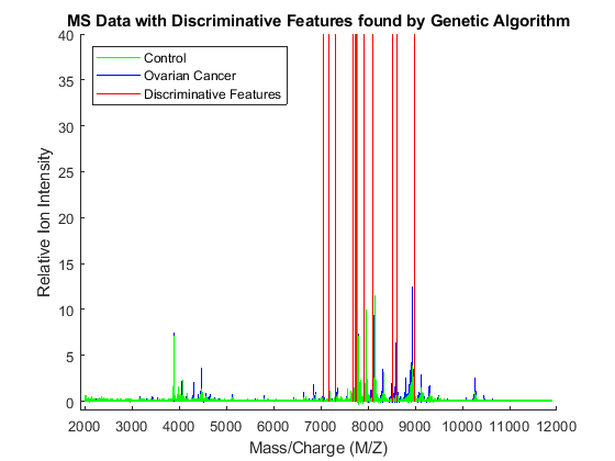
To visualize which features have been selected by the genetic algorithm, the data is plotted with peak positions marked with red vertical lines.

xAxisLabel = 'Mass/Charge (M/Z)';       % x label for plots
yAxisLabel = 'Relative Ion Intensity';  % y label for plots
figure; hold on;
hC = plot(MZ,Y(:,1:15) ,'b');
hN = plot(MZ,Y(:,141:155),'g');
hG = plot(MZ(feat(ceil((1:3*nVars )/3))), repmat([0 100 NaN],1,nVars),'r');
xlabel(xAxisLabel); ylabel(yAxisLabel);
axis([1900 12000 -1 40]);
legend([hN(1),hC(1),hG(1)],{'Control','Ovarian Cancer', 'Discriminative Features'}, ...
    'Location', 'NorthWest');
title('MS Data with Discriminative Features found by Genetic Algorithm');

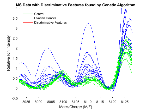
Observe the interesting peak around 8100 Da., which seems to be shifted to the right on healthy samples.

axis([8082 8128 -.5 4])

References

[1] Conrads, T P, V A Fusaro, S Ross, D Johann, V Rajapakse, B A Hitt, S M Steinberg, et al. “High-Resolution Serum Proteomic Features for Ovarian Cancer Detection.” Endocrine-Related Cancer, June 2004, 163–78.

[2] Petricoin, Emanuel F, Ali M Ardekani, Ben A Hitt, Peter J Levine, Vincent A Fusaro, Seth M Steinberg, Gordon B Mills, et al. “Use of Proteomic Patterns in Serum to Identify Ovarian Cancer.” The Lancet 359, no. 9306 (February 2002): 572–77.